Excel Templates to accompany Operations Management, Eleventh Edition
created by Lee Tangedahl
Copyright © 2012 by The McGraw Hill Companies, Inc. All rights reserved.
Chapter Eighteen – Management of Waiting Lines
Templates: Single Channel Waiting Line Model (B) Example 3
Lecture Suggestions Solved Problems: Solved Problem 1
Solved Problem 3
Example 2 Problems Problems 1-9
Problems 10-17
See Instructions template for complete instructions.
Multiple Channel Waiting Line Model (B) Example 4
Multiple Priorities Waiting Line Model (B) Example 5
Example 9
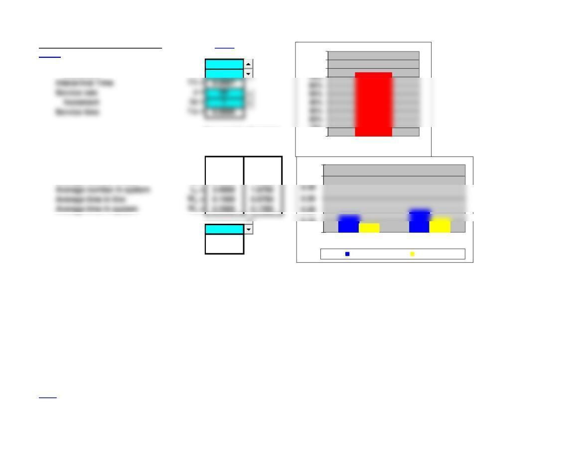
Single Channel Waiting Line Model Basic
<Back
Arrival rate l = 15
Increment Dl = 1
Exponential
Constant
Service Service
Time Time
System Utilization r = 0.7500 0.7500 Wq
Probability system is empty P0 = 0.2500 0.2500 Ws
Average number in line Lq = 2.2500 1.1250 0.9
Average number in system Ls = 3.0000 1.8750 18
Average time in line Wq = 0.1500 0.0750 20
Average time in system Ws = 0.2000 0.1250 0.9
n = 4 9
P( 4 units in system) P( 4 ) = 0.0791 0.45
P( < 4 units in system ) P( < 4) = 0.6836 0.5
Basic Template: You can simply copy the basic template below and paste into another worksheet.
^Top
0%
10%
80%
90%
100%
System Utilization
0.00
0.10
0.50
0.60
Wq Ws
Exponential Constant
Interarrival Time 1/l = 0.0667
Service rate m = 20
Increment Dm = 1
Service time 1/m = 0.0500
Single Channel Waiting Line Model
Arrival rate l = 15
Exponential
Constant
Service Service
Time Time
System Utilization r = 0.7500 0.7500
Probability system is empty P0 = 0.2500 0.2500
Average number in line Lq = 2.2500 1.1250
Average number in system Ls = 3.0000 1.8750
Average time in line Wq = 0.1500 0.0750
P( 4 units in system) P( 4 ) = 0.0791
Interarrival Time 1/l = 0.0667
Service rate m = 20
Service time 1/m = 0.0500
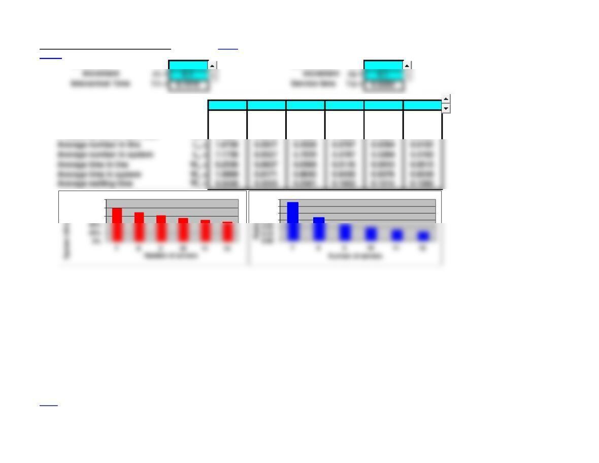
Multiple Channel Waiting Line Model Basic
<Back
Arrival rate l = 6.6 Service rate m = 1.2
Number of servers (max 12) M = 7 8 9 10 11 12
System Utilization r = 0.7857 0.6875 0.6111 0.5500 0.5000 0.4583
Probability system is empty P0 = 0.0032 0.0038 0.0040 0.0040 0.0041 0.0041
Probability arrival must wait Pw = 0.4564 0.2512 0.1298 0.0628 0.0284 0.0121
Average number in line Lq = 1.6736 0.5527 0.2039 0.0767 0.0284 0.0102
Average number in system Ls = 7.1736 6.0527 5.7039 5.5767 5.5284 5.5102
Average time in line Wq = 0.2536 0.0837 0.0309 0.0116 0.0043 0.0015
Average time in system Ws = 1.0869 0.9171 0.8642 0.8450 0.8376 0.8349
Basic Template: You can simply copy the basic template below and paste into another worksheet.
^Top
60%
80%
100%
0.30
0.40
0.50
0.60
Interarrival Time 1/l = 0.1515 Service time 1/m = 0.8333
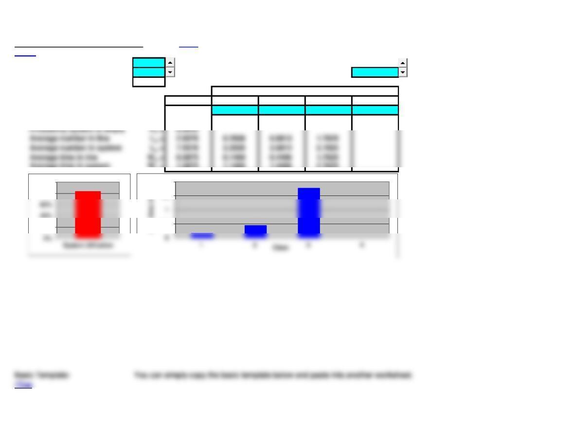
Multiple Channel Waiting Line Model
Arrival rate l = 6.6 Calculations:
321.625 -33.275 -0.086
Number of servers (max 12) M = 7 449.354 -101.674 -0.019
System Utilization r = 0.7857 587.482 -419.404 -0.003
Probability system is empty P0 = 0.0032 6129.422 461.344 0.002
Probability arrival must wait Pw = 0.4564 7167.867 140.966 0.003
Average number in line Lq = 1.6736 8198.075 66.456 0.004
Average number in system Ls = 7.1736 9218.842 32.634 0.004
Average time in line Wq = 0.2536 10 231.533 15.511 0.004
Average time in system Ws = 1.0869 11 238.513 6.980 0.004
Interarrival Time 1/l = 0.1515 M P0
Service rate m = 1.2 11.000 -1.222 -4.500
Service time 1/m = 0.8333 26.500 -8.643 -0.467
Calculations:
l = 6.6
m = 1.2
M P0
11.000 -1.222 -4.500
321.625 -33.275 -0.086
587.482 -419.404 -0.003
7167.867 140.966 0.003
9218.842 32.634 0.004
11 238.513 6.980 0.004
12 242.003 2.953 0.004
Multiple Priorities Waiting Line Model Basic
<Back
Service rate m = 1
Increment Dm = 1 Number of servers M = 6
Service time 1/m = 1.0000
Class
System 1 2 3 4
Arrival rate l = 5.0000 2 2 1
System Utilization r = 0.8333
Average time in system Ws = 1.5875 1.1469 1.4406 2.7625
20%
80%
100%
0.5
1.5
2
Ave. time in line
Multiple Priorities Waiting Line Model
Service rate m = 1 Calculations:
11.000 -1.250 -4.000
Class 26.000 -8.333 -0.429
System 1 2 3 318.500 -31.250 -0.078
Arrival rate l = 5.0000 2 2 1 439.333 -104.167 -0.015
System Utilization r = 0.8333 565.375 #DIV/0! #DIV/0!
11 146.381 2.243 0.007
12 147.604 0.874 0.007
Service time 1/m = 1.0000
Calculations:
lamda = 5
mu = 1
M P0
11.000 -1.250 -4.000
26.000 -8.333 -0.429
439.333 -104.167 -0.015
691.417 130.208 0.005
8128.619 25.835 0.006
10 143.689 5.382 0.007
12 147.604 0.874 0.007
Finite Source Waiting Line Model Basic
<Back
Population Size N = 5 5
Number of servers M = 1 2
Average service time T = 10 10
Average time between service calls U = 70 70
Per Time
Unit
Service cost = 10 10 20
Basic Template: You can simply copy the basic template below and paste into another worksheet.
^Top
P(wait) – from table D = 0.4730 0.0820
Efficiency factor – from table F = 0.9200 0.9940
Average number waiting L = 0.4000 0.0300
Average waiting time W = 6.9565 0.4829
Average number running J = 4.0250 4.3488
Average number being serviced H = 0.5750 0.6213
Finite Source Waiting Line Model
Population Size N = 5 5
Number of servers M = 1 2
Average service time T = 10 10
Average time between service calls U = 70 70
Per Time
Unit
Service cost = 10 10 20
P(wait) – from table D = 0.4730 0.0820
Efficiency factor – from table F = 0.9200 0.9940
Average number waiting L = 0.4000 0.0300
Average waiting time W = 6.9565 0.4829
Average number running J = 4.0250 4.3488
Average number being serviced H = 0.5750 0.6213
Lecture Suggestions – Chapter 18
<Back
Example 2: Single Channel Waiting Line Model
1. Select the Example 2 worksheet
3.
Enter service rate m = 20, point out the average service time = 1 / m = .0500.
Discuss the queuing performance measures.
5.
Compare the system having exponential service times (first column) with the system having a
constant service time (second column).
Demonstrate that the table at the bottom will compute the probability of n in the system (i.e. the
7.
Use the spinner buttons beside l and m to demonstrate the effect of changing l and/or m. For
example, as the value of l approaches the value of m, the system utilization goes up and the time
in the line and in the system go up (see graphs).
Enter arrival rate l = 15, point out the average interarrival time = 1 / l = .0667.
Multiple Channel Waiting Line Model
<Back
Arrival rate l = 18 Service rate m = 20
Increment Dl = 1 Increment Dm = 1
Interarrival Time 1/l = 0.0556 Service time 1/m = 0.0500
Number of servers (max 12) M = 1 2 3 4 5 6
System Utilization r = 0.9000 0.4500 0.3000 0.2250 0.1800 0.1500
0%
40%
60%
80%
100%
0.00
0.30
0.40
0.50
0.60
1 2 3 4 5 6
Calculations:
l = 18
m = 20
M P0
21.900 0.736 0.379
42.427 0.035 0.406
62.459 0.001 0.407
82.460 0.000 0.407
10 2.460 0.000 0.407
12 2.460 0.000 0.407
Single Channel Waiting Line Model
<Back
Arrival rate l = 15
Increment Dl = 1
Interarrival Time 1/l = 0.0667
Exponential
Constant
Service Service
Time Time
System Utilization r = 0.7500 0.7500 Wq
Probability system is empty P0 = 0.2500 0.2500 Ws
Average number in line Lq = 2.2500 1.1250 0.9
Average number in system Ls = 3.0000 1.8750 18
Average time in line Wq = 0.1500 0.0750 20
Average time in system Ws = 0.2000 0.1250 0.9
8.1
n = 4 9
0%
10%
70%
80%
90%
100%
System Utilization
0.10
0.50
0.60
Service rate m = 20
Increment Dm = 1
Service time 1/m = 0.0500
Single Channel Waiting Line Model
<Back
Arrival rate l = 8
Increment Dl = 1
Interarrival Time 1/l = 0.1250
Exponential
Constant
Service Service
Time Time
System Utilization r = 0.6667 0.6667 Wq
Probability system is empty P0 = 0.3333 0.3333 Ws
Average number in line Lq = 1.3333 0.6667 0.9
Average number in system Ls = 2.0000 1.3333 18
Average time in line Wq = 0.1667 0.0833 20
Average time in system Ws = 0.2500 0.1667 0.9
n = 4 9
P( 4 units in system) P( 4 ) = 0.0658 0.45
0%
10%
20%
60%
70%
80%
90%
100%
System Utilization
0.00
0.10
0.60
Service rate m = 12
Increment Dm = 1
Service time 1/m = 0.0833
Multiple Channel Waiting Line Model
<Back
Arrival rate l = 6.6 Service rate m = 1.2
Increment Dl = 0.1 Increment Dm = 0.1
Interarrival Time 1/l = 0.1515 Service time 1/m = 0.8333
Number of servers (max 12) M = 7 8 9 10 11 12
System Utilization r = 0.7857 0.6875 0.6111 0.5500 0.5000 0.4583
Probability system is empty P0 = 0.0032 0.0038 0.0040 0.0040 0.0041 0.0041
60%
80%
100%
0.40
0.50
0.60
Probability arrival must wait Pw = 0.4564 0.2512 0.1298 0.0628 0.0284 0.0121
Average number in line Lq = 1.6736 0.5527 0.2039 0.0767 0.0284 0.0102
Average number in system Ls = 7.1736 6.0527 5.7039 5.5767 5.5284 5.5102
Average time in line Wq = 0.2536 0.0837 0.0309 0.0116 0.0043 0.0015
Average time in system Ws = 1.0869 0.9171 0.8642 0.8450 0.8376 0.8349
Calculations:
l = 6.6
m = 1.2
M P0
26.500 -8.643 -0.467
449.354 -101.674 -0.019
6129.422 461.344 0.002
8198.075 66.456 0.004
10 231.533 15.511 0.004
12 242.003 2.953 0.004
Multiple Channel Waiting Line Model
<Back
Arrival rate l = 4.8 Service rate m = 1.5
Increment Dl = 0.1 Increment Dm = 0.1
Interarrival Time 1/l = 0.2083 Service time 1/m = 0.6667
Number of servers (max 12) M = 4 5 6 7 8 9
System Utilization r = 0.8000 0.6400 0.5333 0.4571 0.4000 0.3556
Probability system is empty P0 = 0.0273 0.0372 0.0398 0.0405 0.0407 0.0407
Probability arrival must wait Pw = 0.5964 0.2886 0.1271 0.0509 0.0185 0.0061
Average waiting time Wa = 0.8333 0.3704 0.2381 0.1754 0.1389 0.1149
80%
100%
0.80
1.00
Average number in line Lq = 2.3857 0.5130 0.1453 0.0428 0.0123 0.0034
Average number in system Ls = 5.5857 3.7130 3.3453 3.2428 3.2123 3.2034
Average time in line Wq = 0.4970 0.1069 0.0303 0.0089 0.0026 0.0007
Average time in system Ws = 1.1637 0.7735 0.6969 0.6756 0.6692 0.6674
Calculations:
l = 4.8
m = 1.5
M P0
11.000 -1.455 -2.200
39.320 -81.920 -0.014
519.150 7.767 0.037
723.438 1.256 0.040
924.392 0.150 0.041
11 24.520 0.013 0.041