17 – 1
Chapter 17
Markov Processes
Learning Objectives
1. Learn about the types of problems that can be modeled as Markov processes.
4. Know what is meant by the steady-state probabilities.
5. Know how to solve Markov processes models having absorbing states.
6. Understand the following terms:
state of the system
Markov Processes
17 – 1
Solutions:
1.
State
Large
Probability
0
1
2
3
4
5
6
7
8
9
10
→ n
1 (n)
0.5
0.55
0.585
0.610
0.627
0.639
0.647
0.653
0.657
0.660
0.662
→ 2/3
2 (n)
2. a.
b. 1 = 0.5, 2 = 0.5
c. 𝑃=[0.90 0.10
0.10 0.85] 𝜋1=.6 𝜋2=.4
3. a. 0.10
b. 1 = 0.75, 2 = 0.25
4. a. 1 = 0.92, 2 = 0.08
5.
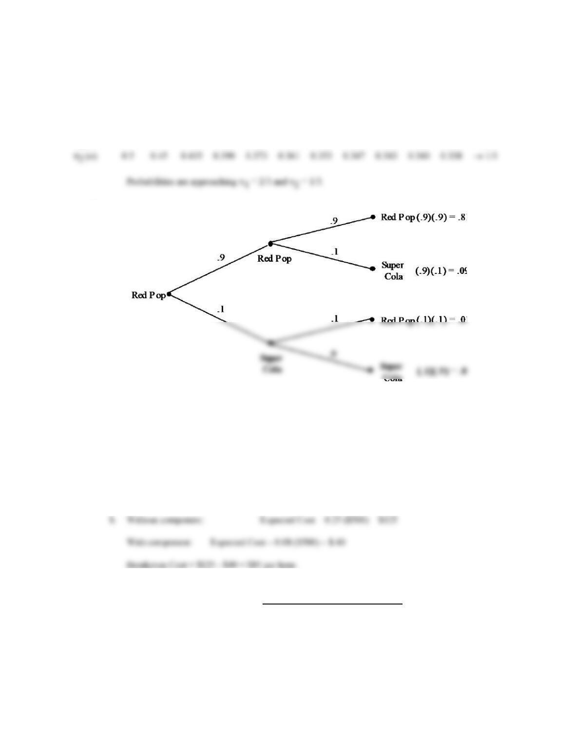
No T raffic Delay
0.85
0.25
T raffic Delay
0.15
0.75
No T raffic Delay
T raffic Delay
Chapter 17
17 –
2
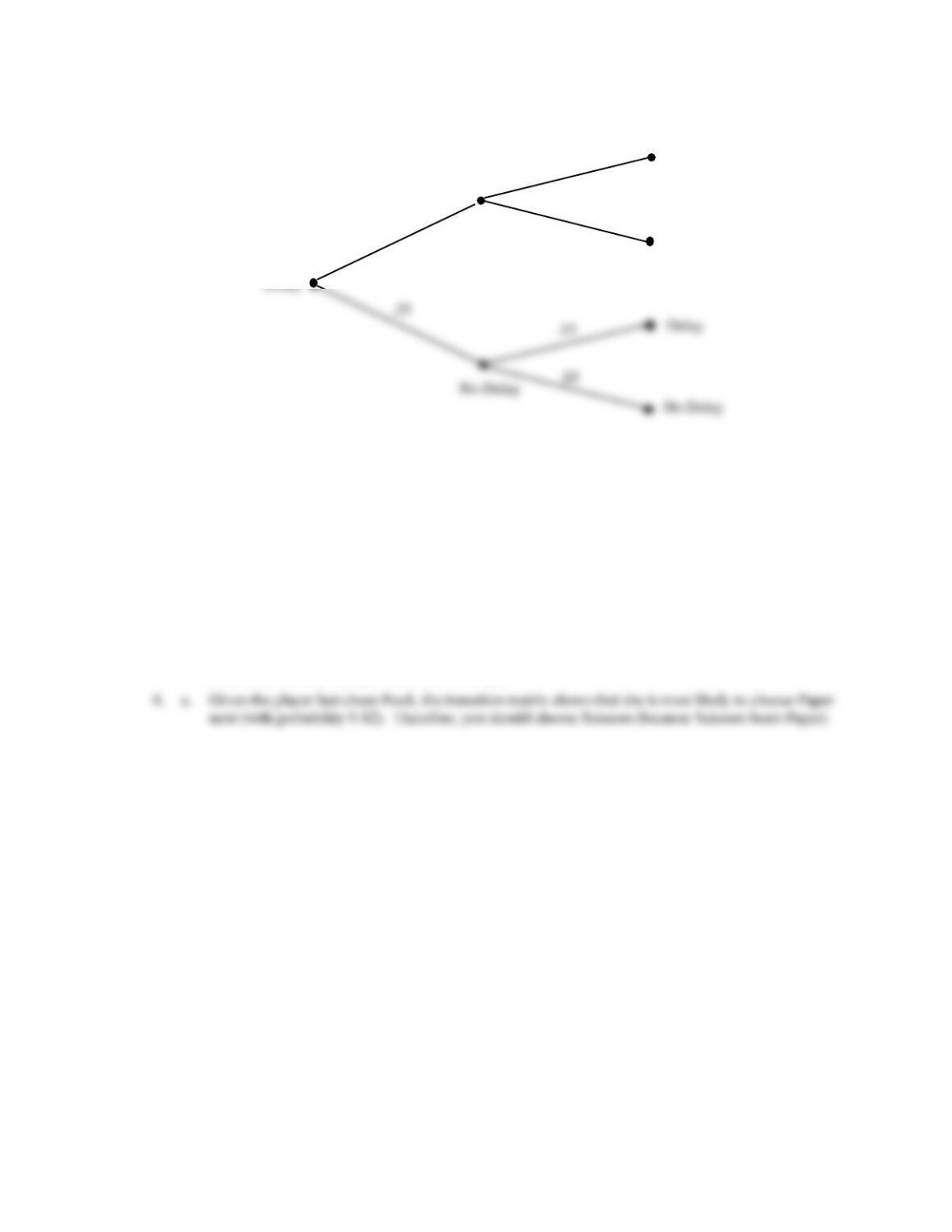
a.
Delay
Delay
No Delay
.75
.75
.25
P (Delay 60 minutes) = (0.75)(0.75) = 0.5625
b. 1 = 0.85 1 + 0.25 2
2 = 0.15 1 + 0.75 2
1 + 2 = 1
Solve for 1 = 0.625 and 2 = 0.375
c. This assumption may not be valid. The transition probabilities of moving to delay and no delay
states may actually change with the time of day.
17 –
3
b.
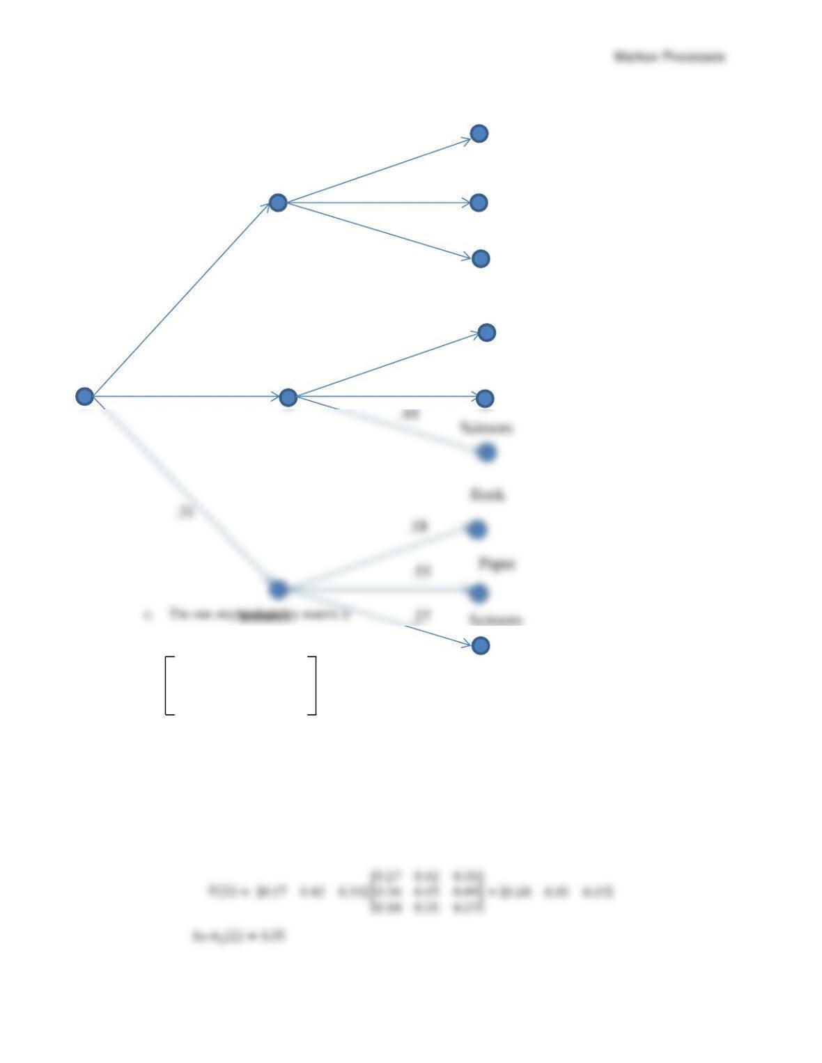
Scissors
Scissors
Rock
Paper
Scissors
.31
.49
.18
.55
.27
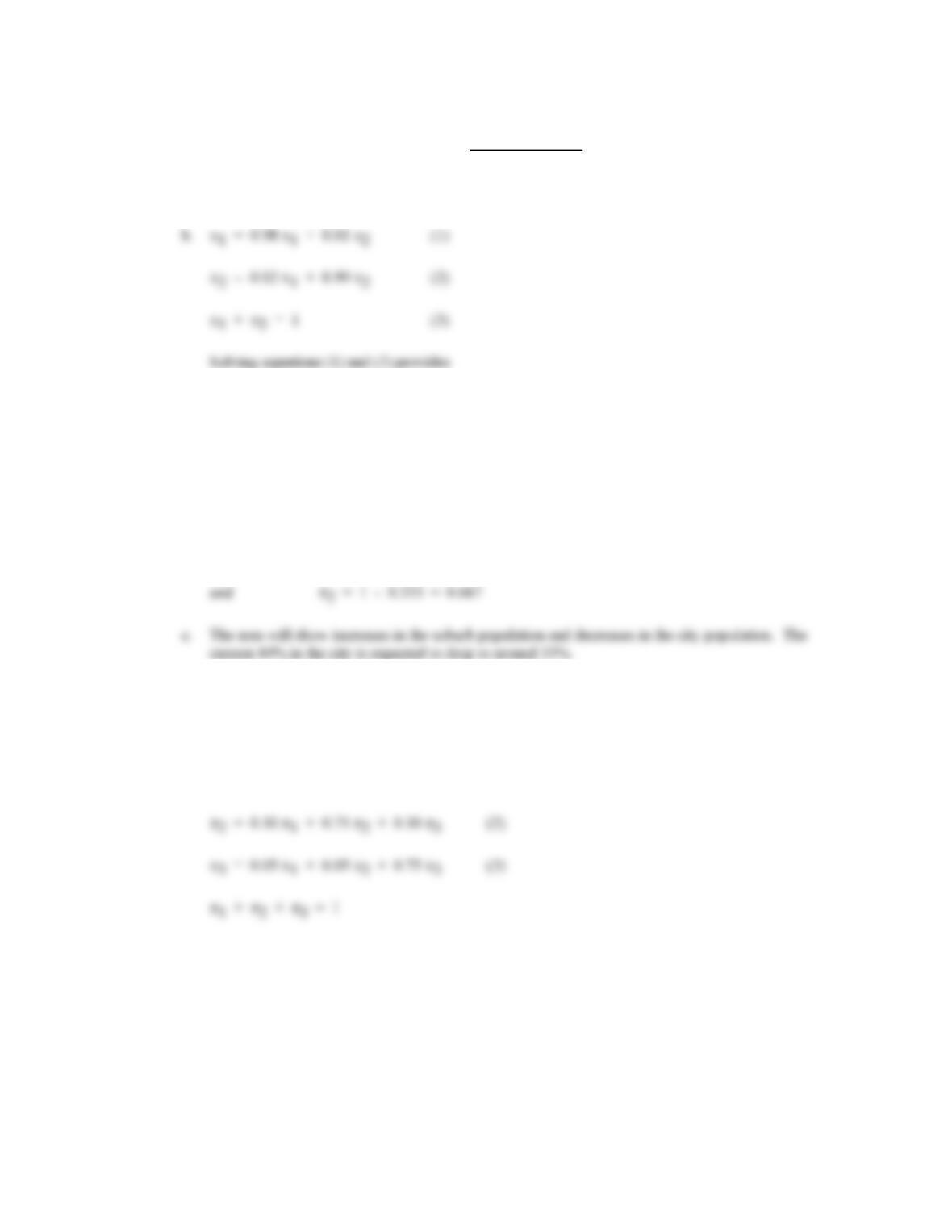
0.27 0.42 0.31
P = 0.36 0.15 0.49
0.18 0.55 0.27
The probability your opponent will choose Paper in the second round is given by 𝜋2(2). This can be
found from Π(2) by first finding Π(1) as shown below.
Π(1)=[1 0 0][0.27 0.42 0.31
0.36 0.15 0.49
0.18 0.55 0.27]=[0.27 0.42 0.31]
Rock
Paper
Rock
Rock
Paper
Scissors
Rock
Paper
.27
.42
.27
.42
.31
.36
.15
Chapter 17
17 –
4
7. a.
0.98
0.01
City
Suburbs
0.02
0.99
City
Suburbs
0.02 1 – 0.01 2 = 0
2 = 1 – 1
Thus, 0.02 – 0.01 (1 – 1) = 0
0.03 1 – 0.01 = 0
1 = 0.333
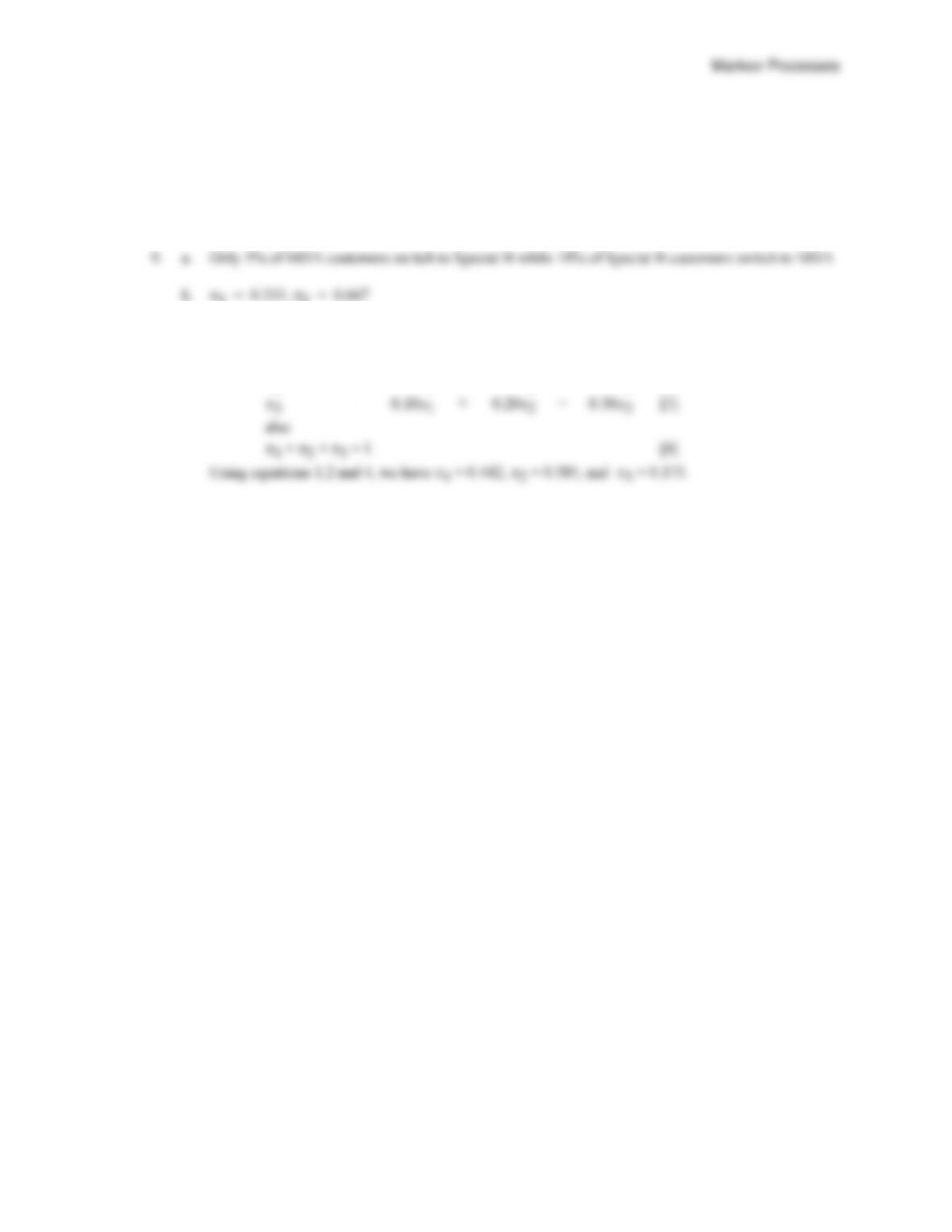
8. a. Let 1 = Murphy’s steady–state probability
2 = Ashley’s steady-state probability
3 = Quick Stop’s steady-state probability
1 = 0.85 1 + 0.20 2 + 0.15 3 (1)
Using 1, 2, and 4 we have
0.15 1 – 0.20 2 – 0.15 3 = 0
-0.10 1 – 0.25 2 – 0.10 3 = 0
1 + 2 + 3 = 1
17 –
5
Solving three equations and three unknowns gives 1 = 0.548, 2 = 0.286, and 3 = 0.166
b. 16.6%
c. Murphy’s 548, Ashley’s 286, and Quick Stop’s 166. Quick Stop should take 667 – 548 = 119
Murphy’s customers and 333 – 286 = 47 Ashley’s customers.
10.
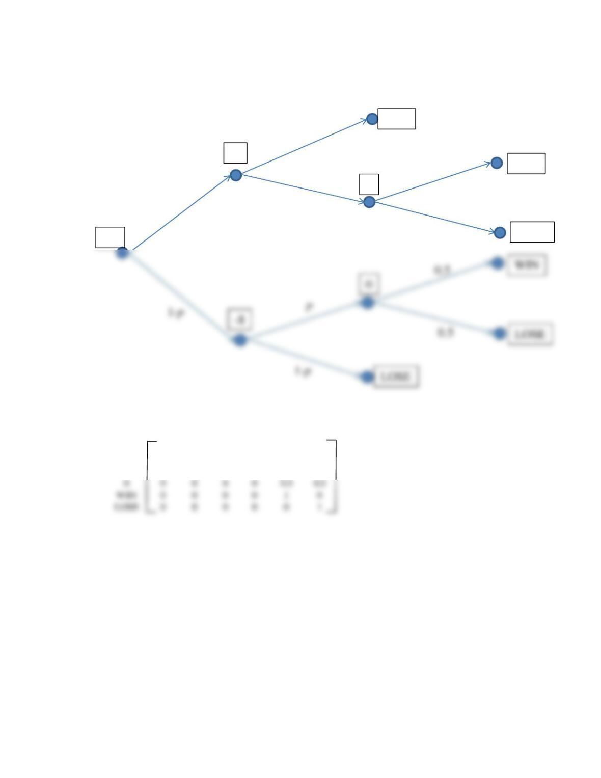
1
=
0.801
+
0.052
+
0.403
[1]
2
=
0.101
+
0.752
+
0.303
[2]
3
=
0.101
+
0.202
+
0.303
[3]
1 + 2 + 3 = 1
[4]
The Markov analysis shows that Special B now has the largest market share. In fact, its market
share has increased by almost 11%. The MDA brand will be hurt most by the introduction of the
new brand, T-White. People who switch from MDA to T-White are more likely to make a second
switch back to MDA.
Chapter 17
17 –
6
11.
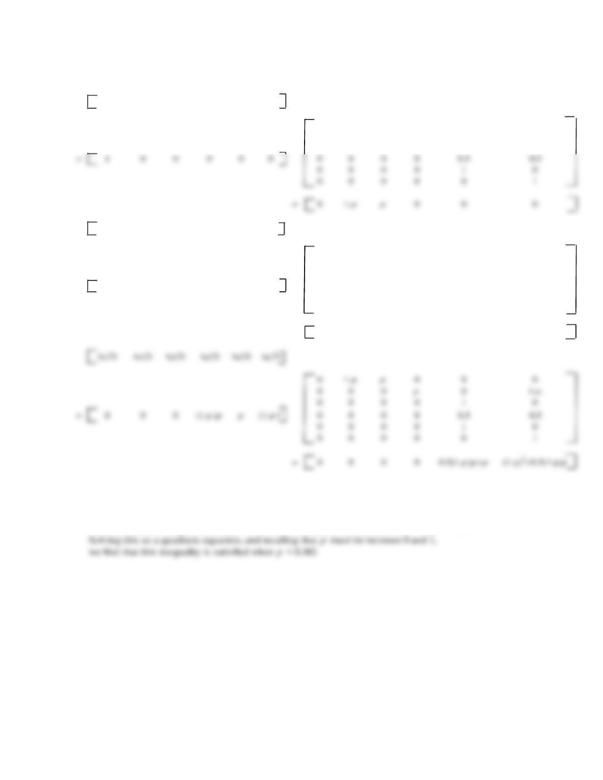
b. Transition Probability Matrix
–14 -8 -6 0 WIN LOSE
–14 0 1-p p 0 0 0
-8 0 0 0 p 0 1-p
-6 0 0 0 0 1 0
a. Tree Diagram
0
LOSE
WIN
1-p
p
1-p
0.5
0.5
-14
-6
WIN
0
p
1
0
0.5
0.5
WIN
LOSE
Markov Processes
17 –
7
c.
1(1) 2(1) 3(1) 4(1) 5(1) 6(1)
0
1-p p 0 0 0
0 0 0 p0
1-p
0 0 0 0 1 0
1-p p 0 0 0
1(2) 2(2) 3(2) 4(2) 5(2) 6(2)
0
1-p p 0 0 0
0 0 0 p0
1-p
0 0 0 0 1 0
= 0
1-p p 0 0 0 0 0 0 0 0.5 0.5
0 0 0 0 1 0
0 0 0 0 0 1
= 0 0 0
(1-p)p p (1-p)2
1-p p 0 0 0
1-p
The probability of winning is 0.5(1–p)p + p = 1.5p – 0.5p2.
Temple’s coach should go for 2 points if this probability is greater than the probability of
winning by going for a one-point conversion after each touchdown, which is 0.5.
Therefore, he should go for a two-point conversion when p is such that 1.5p – 0.5p2 > 0.5.

Chapter 17
17 –
8
12.
13.
14.
15. a. Retirement and leaves for personal reasons are the two absorbing states since both result in the
manager leaving the company.
b. Middle Managers:
Probability of retirement = 0.03
Probability of leaving (personal) = 0.07
c. Senior Managers:
Probability of retirement = 0.08
Probability of leaving (personal) = 0.01
(I–Q) = 1 0
0 1 – 0.4 0.3
0.1 0.5 = 0.6 -0.3
–0.1 0.5
N = (1–Q)
-1
= 1.85 1.11
(I–Q) = 0.7 5 –0.25
–0.05 0.75
N = 1.36 0.45
0.09 1.36
(I–Q) = 0.5 –0.2
0.0 0.5
N = (I–Q)
-1 = 2 0.8
0 2.0
NR = 0.52 0.4 8
0.80 0.2 0
BNR = 150 0 3 500 0.52 0.48
0.80 0.2 0 = 358 0 1 420
17 –
9
d.
55.2% will retire and 44.8% will leave for personal reasons.
16.
a. The Injured and Retired states are absorbing states.
b. Rearrange the transition probability matrix to:
Injured
Retired
Backup
Starter
Injured
1
0
0
0
Retired
0
1
0
0
0.1
I-Q = 0.6 -0.4
-0.1 0.5
N =
(I – Q)-1 = 1.923 1.538
0.385 2.308
38.5% of Starters will eventually be Injured and 61.5% will be Retired.
c.
BNR =[8 5][0.423 0.577
0.385 0.615]=[5.308 7.691]
On average, 5.308 players will end up injured and 7.691 players will retire.
(I-Q) = 1 0
0 1 – 0.80 0.10
0.03 0.88 = 0.20 –0.10
–0.03 0.12
N = (I–Q)
-1 = 5.714 4.762
1.429 9.524
NR = 0.552 0.448
0.805 0.195