Management Chapter 17 Homework Dealer’s Absorbing State Probabilities in Blackjack1.The first step is to create the transition probability matrix for the dealer’s hand

Markov Processes

Chapter 17

Markov Processes

Case Problem: Dealer’s Absorbing State Probabilities in Blackjack

1. The first step is to create the transition probability matrix for the dealer’s hand. The states are defined by the

value of the dealer’s hand after the up card is dealt, and the values the dealer’s hand may assume after the

down card is revealed, and after taking hits. The absorbing states are 17, 18, 19, 20, 21, and bust. According

to the house rules, once the dealer’s hand takes on one of these values she quits taking hits and either pays or

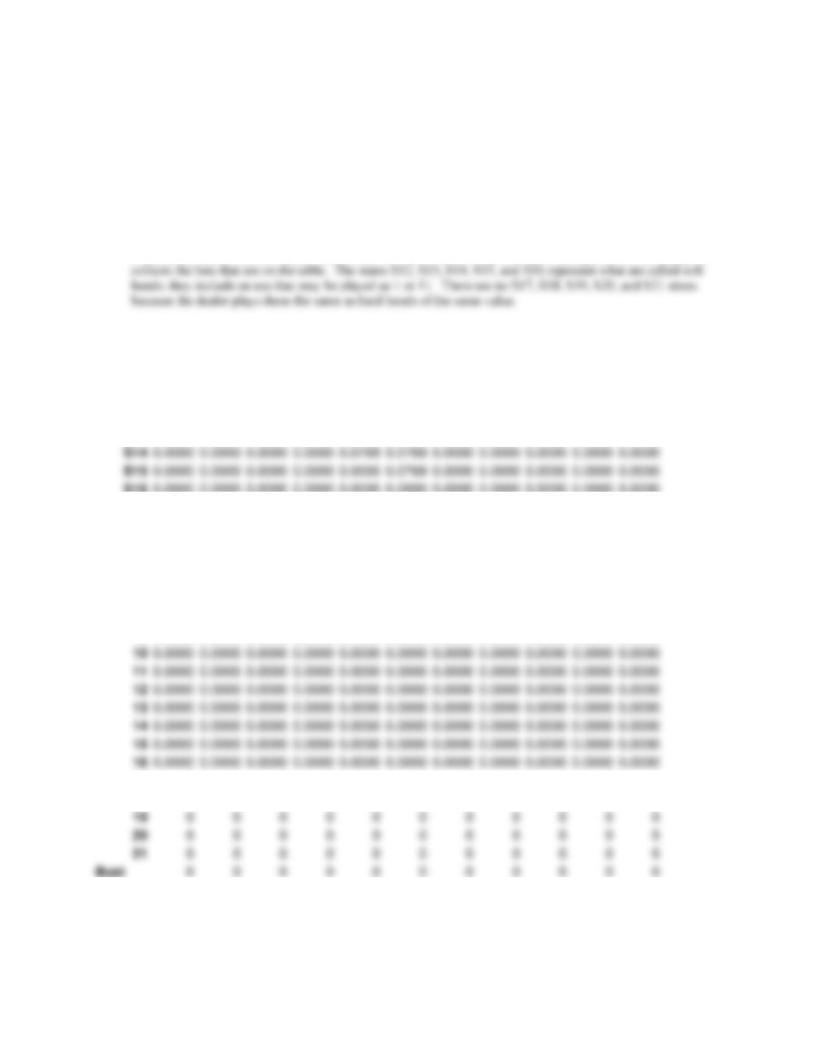
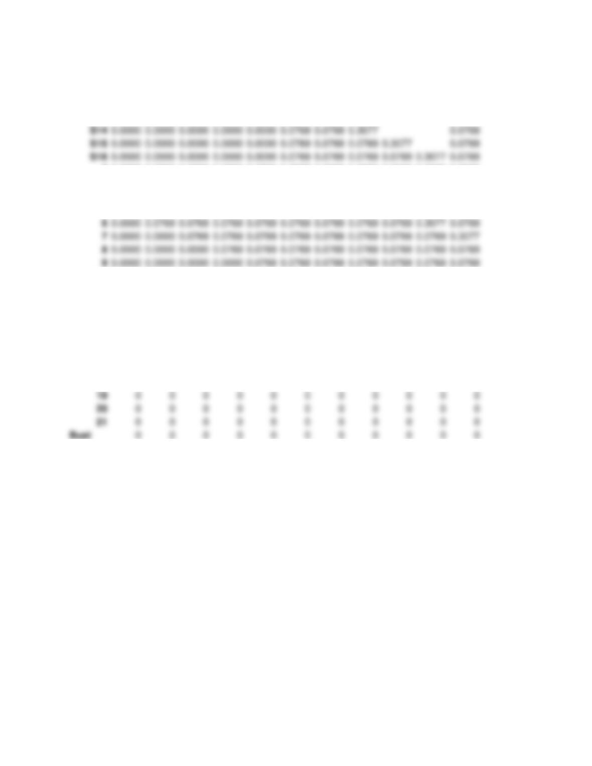
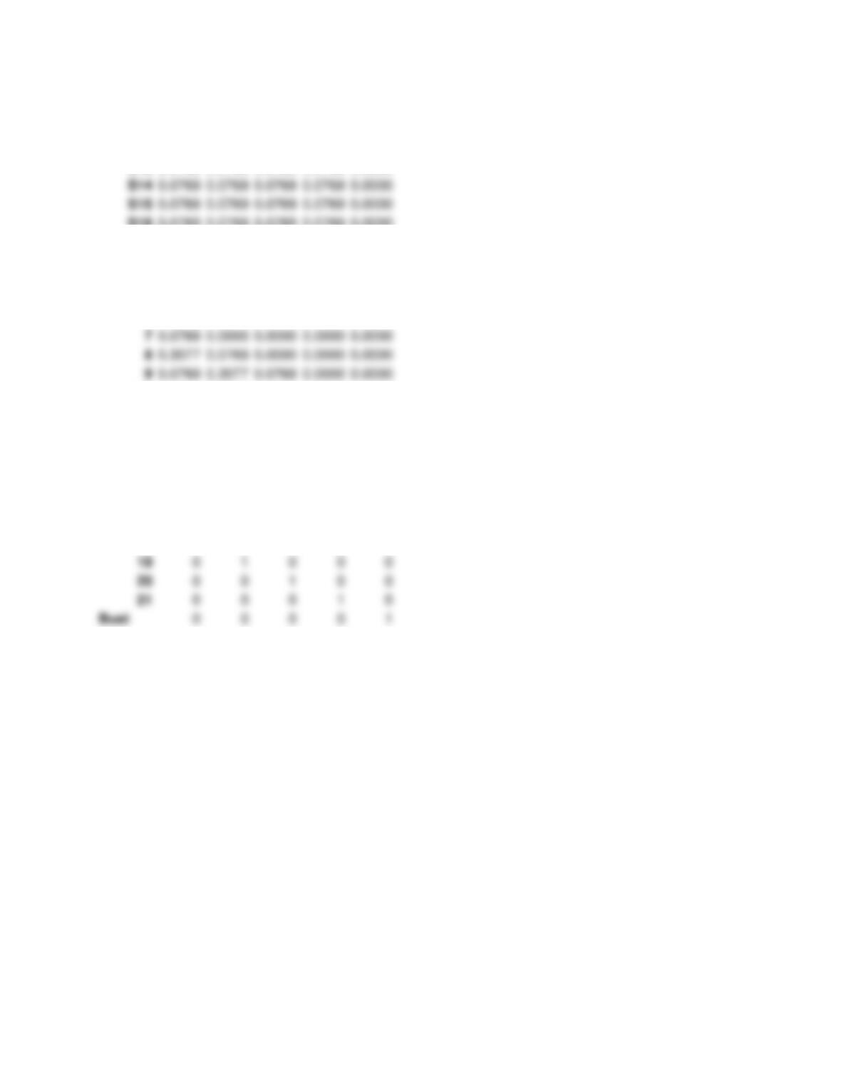
There are 27 states so, due to space restrictions, the transition matrix that is shown below is printed in 3 parts.

All of the rows and a subset of the columns are shown in each part.

A

S12

S13

S14

S15

S16

2

3

4

5

6

A

0.0000

0.0769

0.0000

S12

0.0000

0.0769

0.0000

S13

0.0000

0.0769

0.0000

S14

0.0000

0.0769

0.0000

S15

0.0000

0.0769

0.0000

S16

0.0000

2

0.0000

0.0769

0.0000

0.0769

3

0.0000

0.0769

0.0000

0.0769

4

0.0000

0.0769

0.0000

0.0769

5

0.0000

0.0769

0.0000

6

0.0000

7

0.0000

8

0.0000

9

0.0000

10

0.0000

11

0.0000

12

0.0000

13

0.0000

14

0.0000

15

0.0000

16

0.0000

17

0

18

0

19

0

20

0

21

0

Chapter 17

7

8

9

10

11

12

13

14

15

16

17

A

0.0000

0.0769

S12

0.0000

0.3077

0.0769

S13

0.0000

0.0769

0.3077

0.0769

S14

0.0000

0.0769

0.3077

0.0769

S15

0.0000

0.0769

0.3077

0.0769

S16

0.0000

0.0769

0.3077

0.0769

2

0.0769

0.3077

0.0000

3

0.0769

0.3077

0.0000

4

0.0769

0.3077

0.0000

5

0.0769

0.3077

0.0000

6

0.0000

0.0769

0.3077

0.0769

7

0.0000

0.0769

0.3077

8

0.0000

0.0769

9

0.0000

0.0769

10

0.0000

0.0769

11

0.0000

0.0769

12

0.0000

0.0769

13

0.0000

0.0769

14

0.0000

0.0769

15

0.0000

0.0769

16

0.0000

0.0769

17

0

1

18

0

19

0

20

0

21

0

Markov Processes

18

19

20

21

Bust

A

0.0769

0.3077

0.0000

S12

0.0769

0.0000

S13

0.0769

0.0000

S14

0.0769

0.0000

S15

0.0769

0.0000

S16

0.0769

0.0000

2

0.0000

3

0.0000

4

0.0000

5

0.0000

6

0.0000

7

0.0769

0.0000

8

0.3077

0.0769

0.0000

9

0.0769

0.3077

0.0769

0.0000

10

0.0769

0.3077

0.0769

0.0000

11

0.0769

0.3077

0.0000

12

0.0769

0.3077

13

0.0769

0.3846

14

0.0769

0.4615

15

0.0769

0.5385

16

0.0769

0.6154

17

0

18

1

0

19

0

1

0

20

0

1

0

21

0

1

0

1

Chapter 17

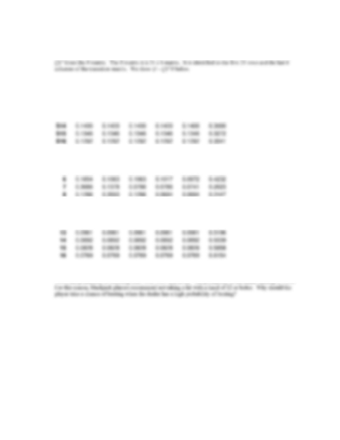
The Q matrix is defined as the first 21 rows (through state 16) and the first 21 columns (through state 16) of

the transition matrix. We must now compute I – Q and (I – Q)-1. We did this using Excel and Excel’s matrix

inversion procedure described in the chapter appendix. To find the absorption probabilities we multiply (I –

Probability of Dealer’s Finishing State Given Starting State

17

18

19

20

21

Bust

A

0.1308

0.3616

0.1153

S12

0.1510

0.2450

S13

0.1455

0.2725

S14

0.1400

0.3000

S15

0.1346

0.3272

S16

0.1292

0.3541

2

0.1398

0.1349

0.1297

0.1240

0.1180

0.3536

3

0.1350

0.1305

0.1256

0.1203

0.1147

0.3739

4

0.1305

0.1259

0.1214

0.1165

0.1112

0.3945

5

0.1223

0.1177

0.1131

0.1082

0.4164

6

0.1654

0.1063

0.1017

0.0972

0.4232

7

0.3686

0.1378

0.0786

0.0741

0.2623

8

0.1286

0.3593

0.1286

0.0694

0.2447

9

0.1200

0.3508

0.1200

0.0608

0.2284

10

0.1114

0.3422

0.1114

0.2121

11

0.1114

0.3422

0.2121

12

0.1035

0.4827

13

0.0961

0.5196

14

0.0892

0.5539

15

0.0828

0.5858

16

0.0769

0.6154

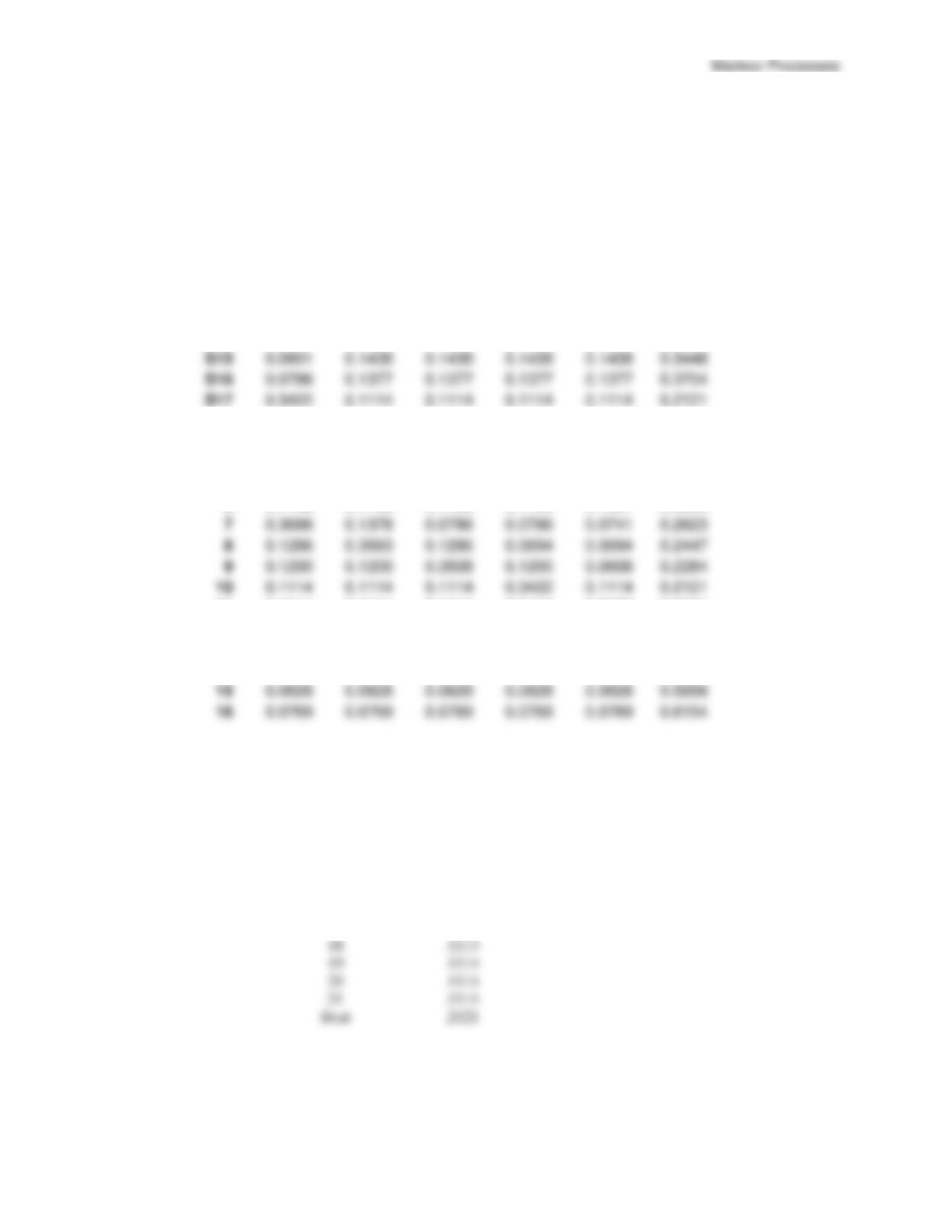
This matrix shows the probabilities for the ending values of the dealer’s hand given any of the starting states

identified by each row. For instance, if the dealer has a 6 as an up card, the probability of finishing with 17 is

2. For this situation another row and column must be added to the transition matrix to account for the soft 17

state, S17. When the dealer has to stay on S17, there was no reason to differentiate soft 17 and hard 17. So

only the state, 17 was used. For space reasons, we do not show the new transition matrix here. But, after

computing (I – Q)-1R, the absorbing state probabilities are given below.

Probability of Dealer’s Finishing State Given Starting State

17

18

19

20

21

Bust

A

0.0575

0.1432

0.3740

0.1389

S12

0.0829

0.1625

0.2669

S13

0.0823

0.1562

0.2929

S14

0.0813

0.1500

0.3189

S15

0.0801

0.1438

0.3448

S16

0.0786

0.1377

0.3704

S17

0.3422

0.1114

0.2121

2

0.1301

0.1365

0.1313

0.1257

0.1196

0.3567

3

0.1263

0.1320

0.1271

0.1218

0.1162

0.3767

4

0.1224

0.1273

0.1228

0.1179

0.1126

0.3971

5

0.1184

0.1229

0.1184

0.1138

0.1089

0.4177

6

0.1148

0.1103

0.1057

0.4395

7

0.3686

0.1378

0.0786

0.0741

0.2623

8

0.1286

0.3593

0.1286

0.0694

0.2447

9

0.1200

0.3508

0.1200

0.0608

0.2284

10

0.1114

0.3422

0.1114

0.2121

11

0.1114

0.3422

0.2121

12

0.1035

0.4827

13

0.0961

0.5196

14

0.0892

0.5539

15

0.0828

0.5858

16

0.0769

0.6154

This matrix shows the probabilities for the ending values of the dealer’s hand given any of the starting states

identified by each row for the case when the dealer hits soft 17. For instance, if the dealer has a 6 as an up

card, the probability of finishing with 17 is .1148, the probability of finishing with 18 is .1148, and so on.

The probability of the dealer busting is .4395.

3. Mathematicians have shown that when the dealer stays on soft 17 it is better for the player. We can provide

the following argument using the finishing values for the dealer’s hand shown in part 2 above. Note that

when the dealer gets S17 and hits it, the finishing values and probabilities for the dealer’s hand are

Ending Value

Probability

17

.3422

18

.1114

19

.1114

20

.1114

21

.1114

.2121

Chapter 17

If the player has 17, the probability of a tie is .3422, the probability of losing is 4(.1114) = .4456, and the

probability of winning is .2121. So, when the player has 17, she will do better (a tie) if the dealer stays on

S17. Similarly, if the player has 18, 19, 20, or 21, she will do much better if the dealer stays on S17. She will

always win.

But, if the player has 12, 13, 14, 15, or 16, she will be better off if the dealer hits soft 17. This is because