Simulation
17 – 1
Chapter 16
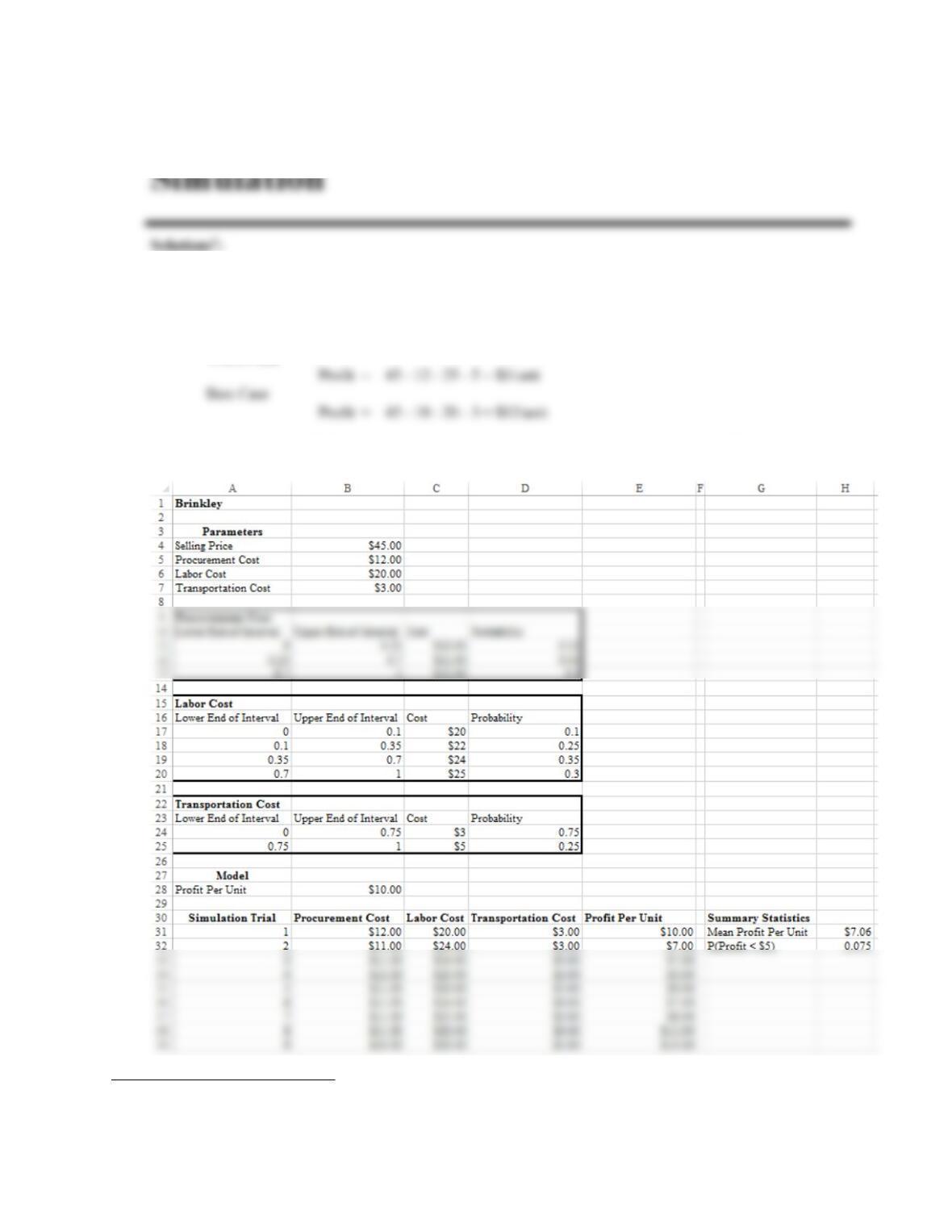
1. a. Profit = Selling Price – Purchase Cost – Labor Cost – Transportation Cost
Base Case using most likely costs
Profit = 45 – 11 – 24 – 3 = $7/unit
b. The average profit from the simulation model (see below) should be approximately $7.06.
1
All solutions are generated with native Excel functionality over 1000 trials per simulation. Simulation results will vary from run
to run.
Chapter 16
16 –
2
c. Simulation will provide a distribution of the profit per unit values. Calculating the percentage of
simulation trials providing a profit less than $5 per unit would provide an estimate of the probability
the profit per unit will be unacceptably low.
d. There is approximately a 0.075 probability that profit per unit will be less than $5.
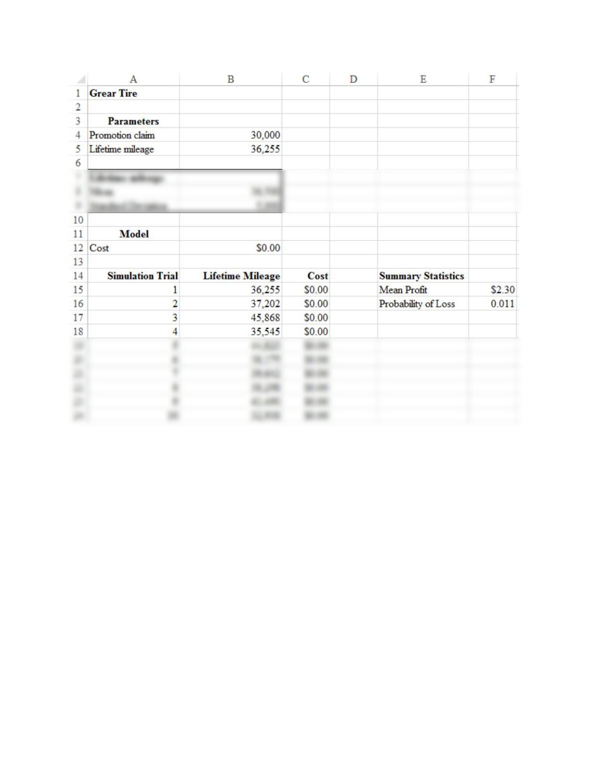
3. a. The average cost of the promotion per tire is approximately $2.30
b. The probability of the refund exceeding $50 is approximately 0.011.
Simulation
16 –
3
c. This question can be answered by trial and error. While the mean profit can vary, a promotion claim
of 29,700 miles will result in an expected cost of approximately $2.00.
Chapter 16
16 –
4
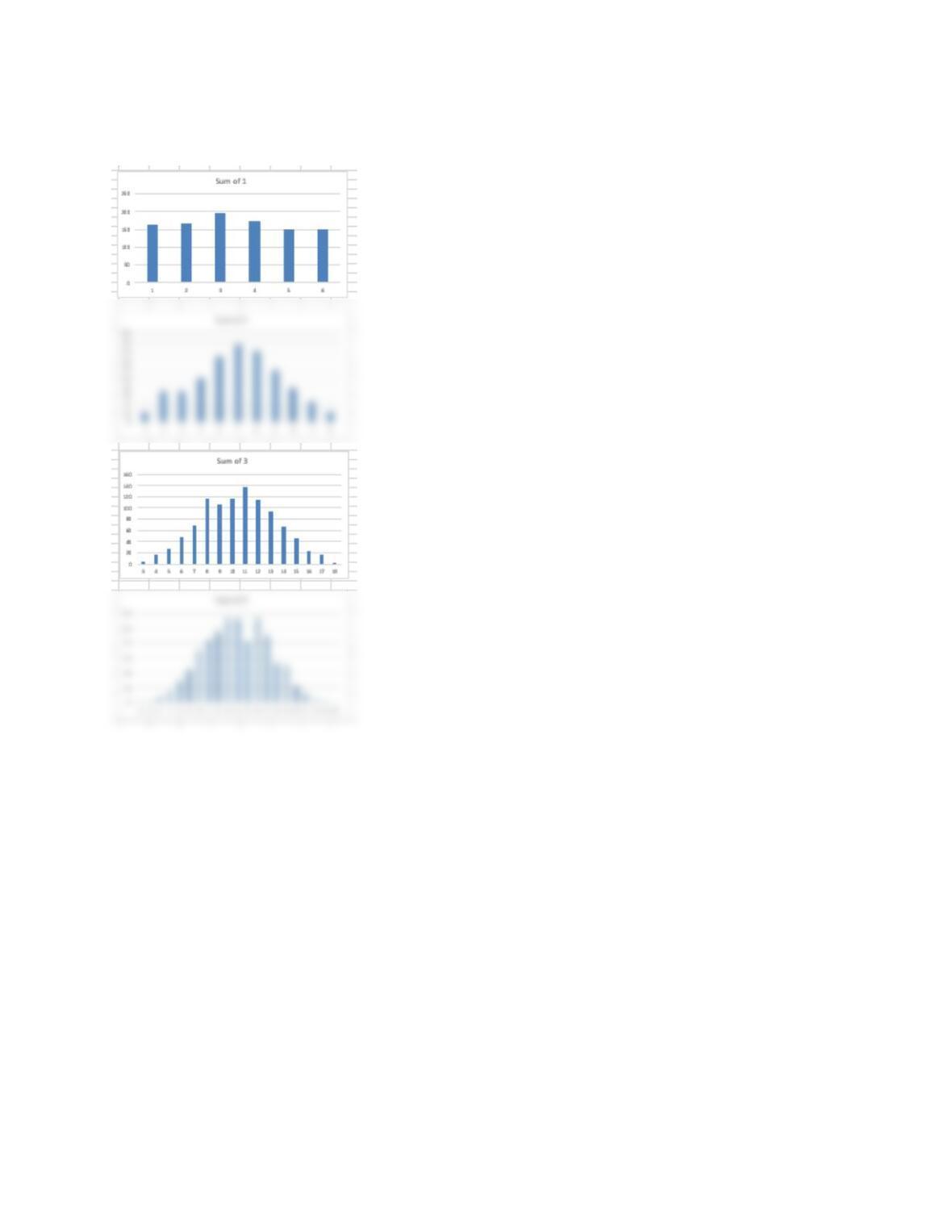
4. As shown in the plots below, as the number of die in the sum increases, the distribution becomes more bell-
shaped. This demonstrates the central limit theorem.
16 –
5
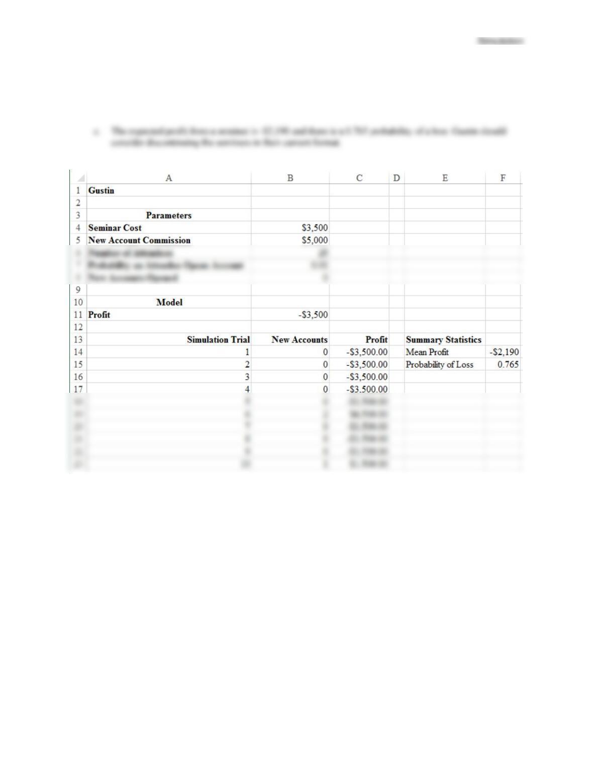
5. a. Profit = (New Accounts Opened × 5000) – 3500
b. The number of new accounts opened is a binomial random variable with 25 trials and 0.01 probability of
a success on a single trial.
d. Trial-and-error shows that, with 70 attendees, the seminar breaks even (the expected profit is very near
$0). Seventy-one attendees are necessary before the expected profit from the seminar is greater than zero
by a non-negible amount.
Chapter 16
16 –
6
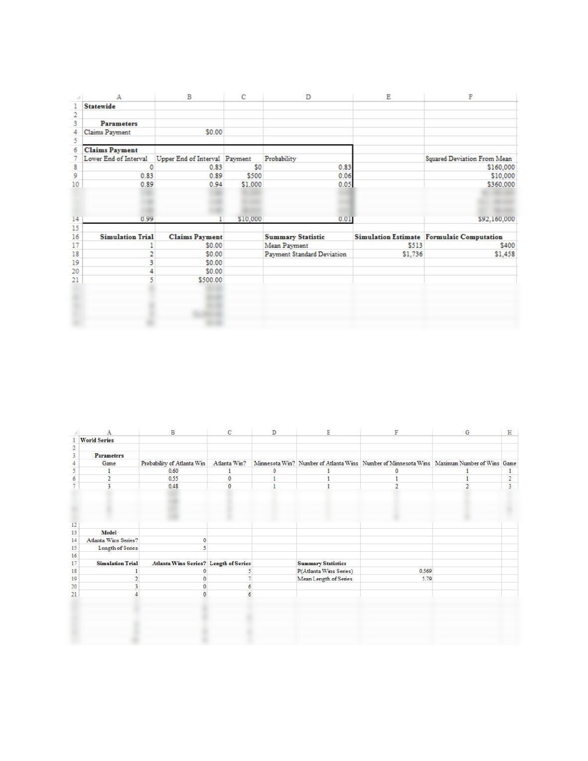
6. a. The screenshot below shows the set of intervals.
b. The simulation-based estimates of the payment mean and standard deviation are $513 and $1736,
respectively. Computing the mean and standard deviation directly from the distribution using the
respective formula, we obtain $400 and $1458, respectively. To reduce the discrepancy between the
simulation-based estimates and the analytical computation, we can increase the number of simulation
trials.
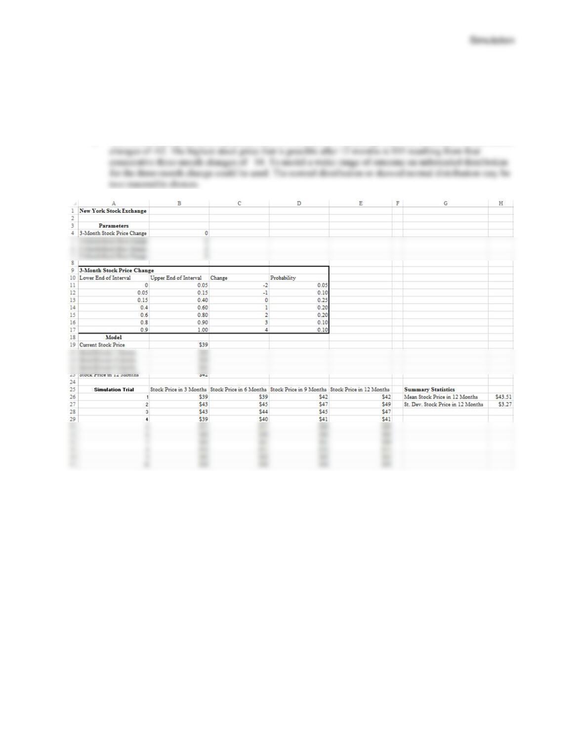
7. a. See screenshot below for example of a spreadsheet model.
b. Atlanta has approximately 0.569 probability of winning the World Series.
16 –
7
c. The expected length of the World Series is approximately 5.79 games.
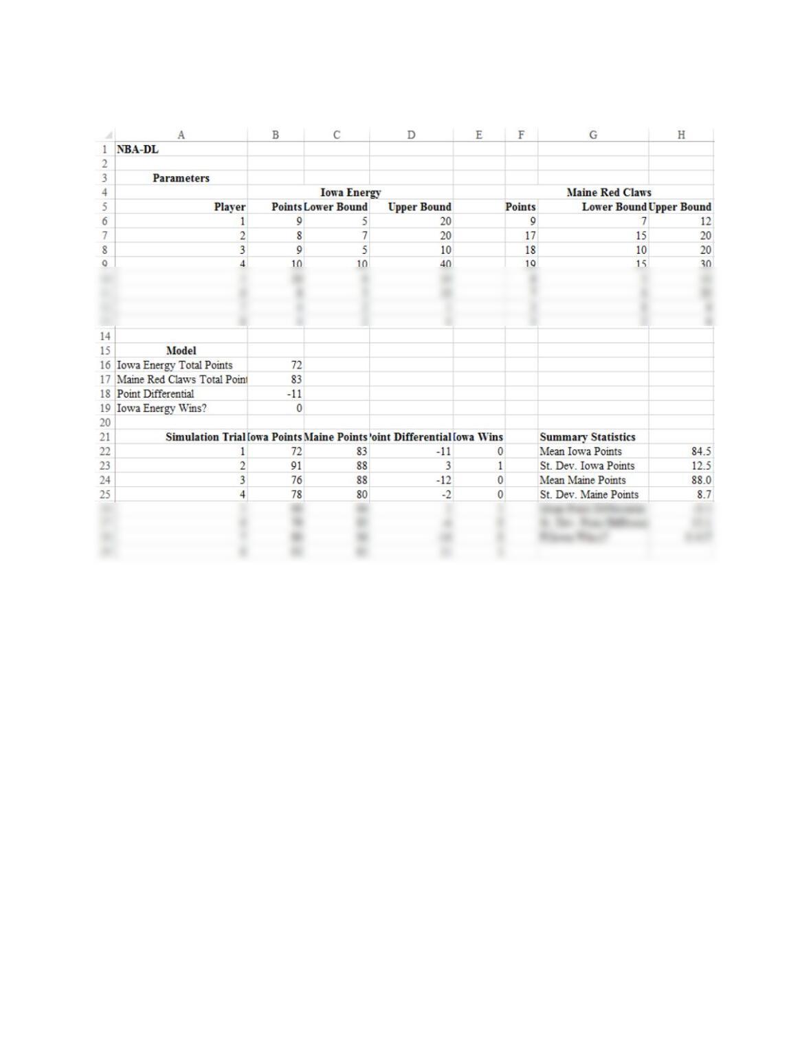
8. a. See screenshot below.
b. The mean stock price after 12 months is $43.51 and the standard deviation is $3.27.
c. The lowest stock price that is possible after 12 months is $31 resulting from four consecutive three-month
Chapter 16
16 –
8
9. a. See screenshot below.
Simulation
16 –
9
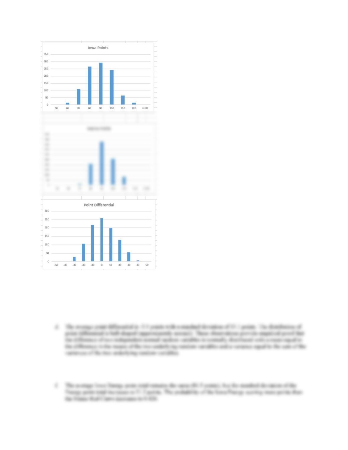
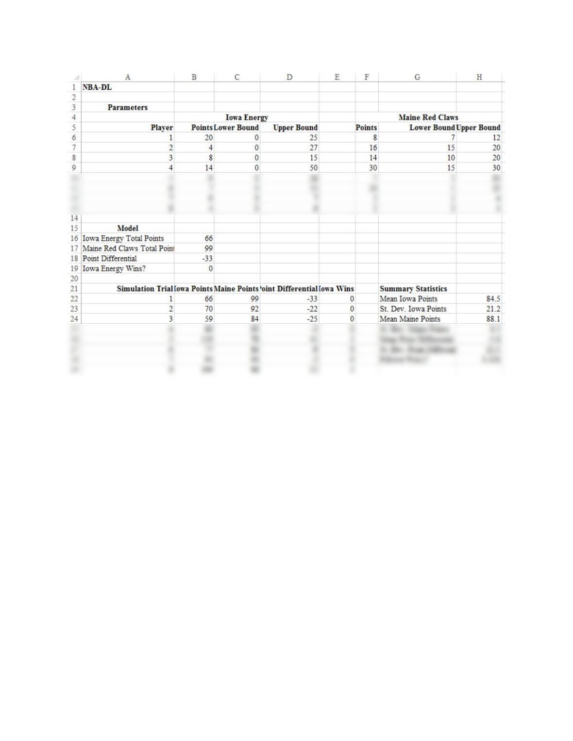
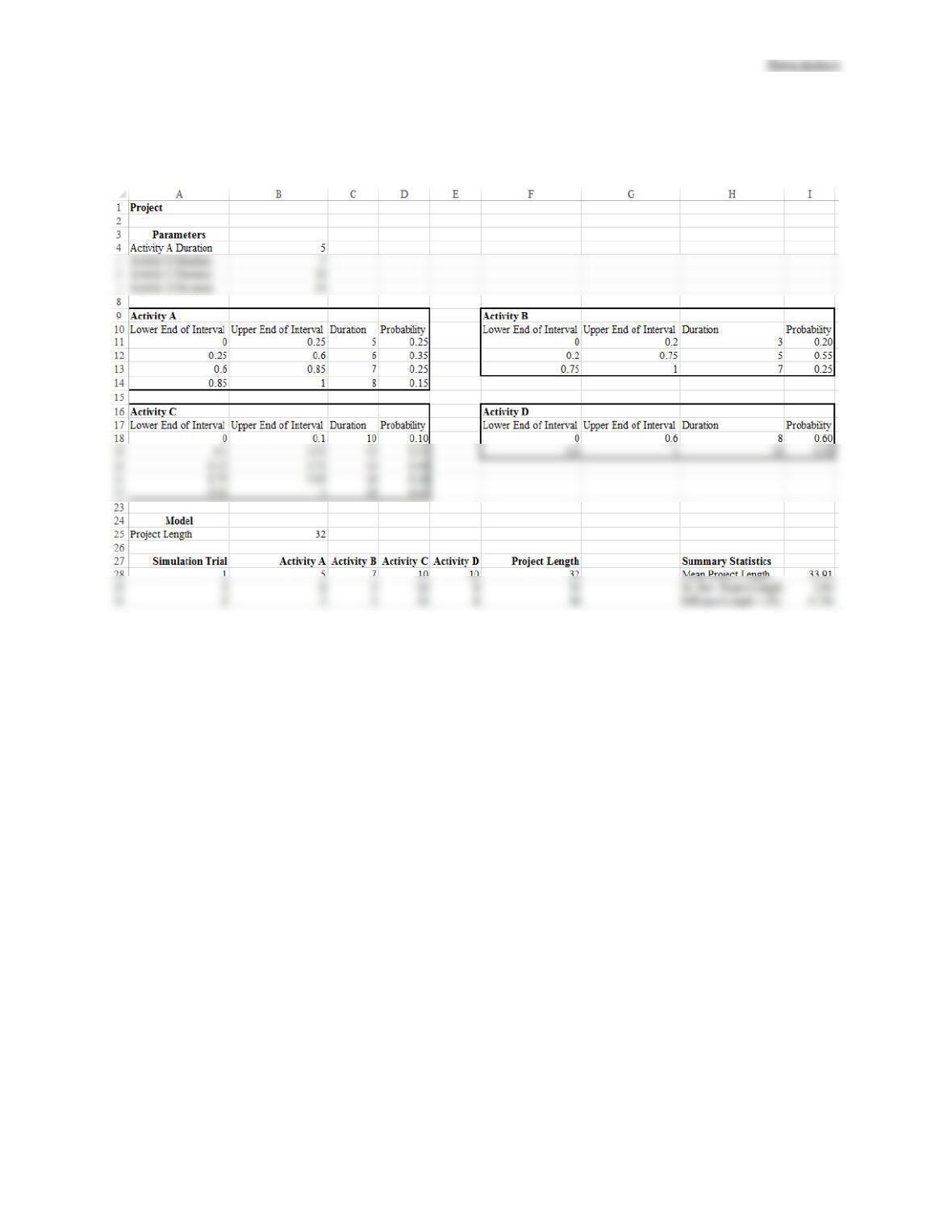
b. The Iowa Energy score an average of approximately 84.5 points with a standard deviation of 12.5 points.
The distribution of points is bell-shaped (approximately normal) as a result of the Central Limit Theorem.
c. The Maine Red Claws score an average of approximately 88.0 points with a standard deviation of 8.7
points. The distribution of points is bell-shaped (approximately normal) as a result of the Central Limit
Theorem.
e. The Iowa Energy has approximately a 0.417 probability of scoring more points than the Maine Red
Claws.
Chapter 16
16 –
10
16 –
11
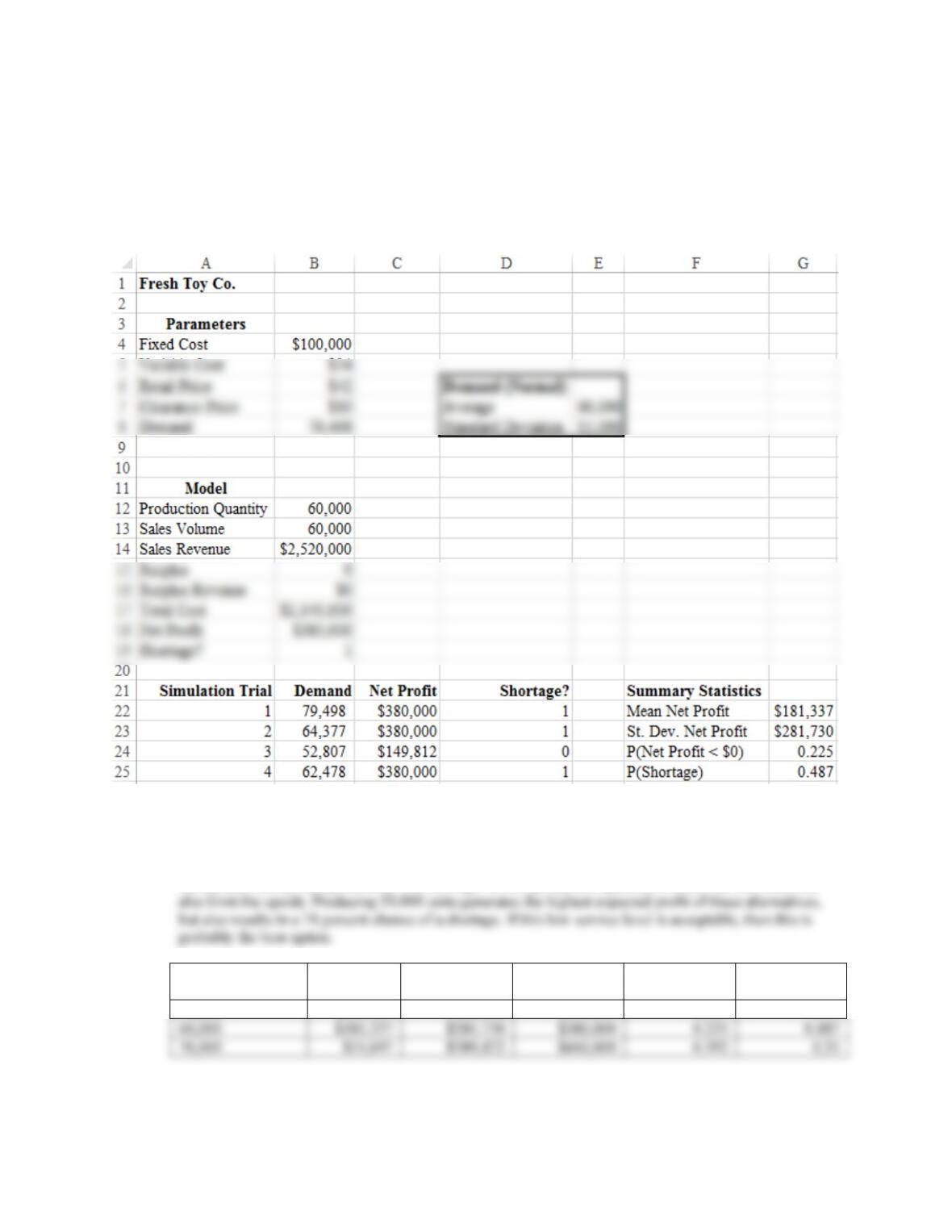
10. a. Expected project length is 33.91 weeks with a standard deviation of 2.81 weeks
b. Probability of completing project in 35 weeks or less is 0.729.
Chapter 16
16 –
12
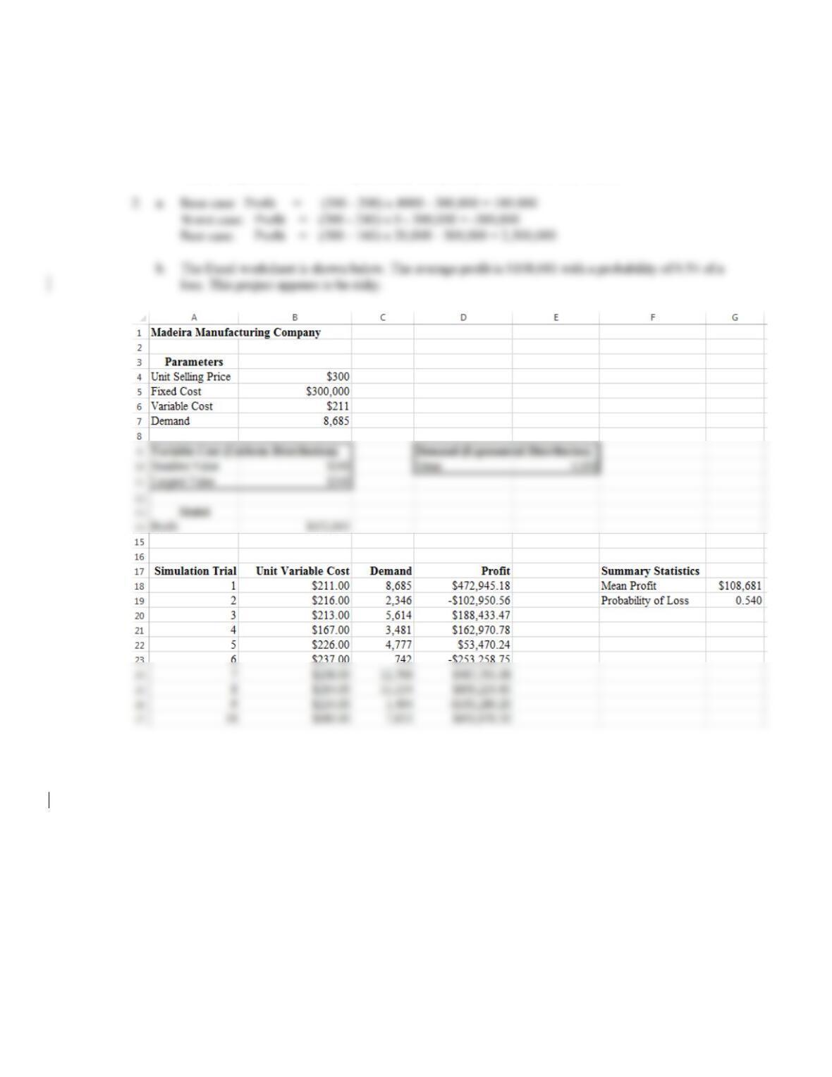
11. a. Profit equals $380,000 when demand is equal to its average of 60,000 units
b. Average profit is approximately $195,381. Average profit is less than the profit corresponding to average
demand. This phenomenon is often called the Flaw of Averages. This occurs because when demand
fluctuates above its average, profit is capped by the order quantity, i.e., there is a ceiling on how much
profit can increase. However, when demand fluctuates below its average, there is no floor on how much
profit can decrease.
c. When ordering 50,000 units, the average profit is approximately $227,814. When ordering 70,000 units,
the average profit is approximately $73,175.
d. Other factors to consider when evaluating a production quantity include: probability of a loss, profit
Production
Quantity
Average
Profit
Profit Standard
Deviation
Maximum
Profit
Probability of
a Loss
Probability of
a Shortage
50,000
60,000
70,000
16 –
13
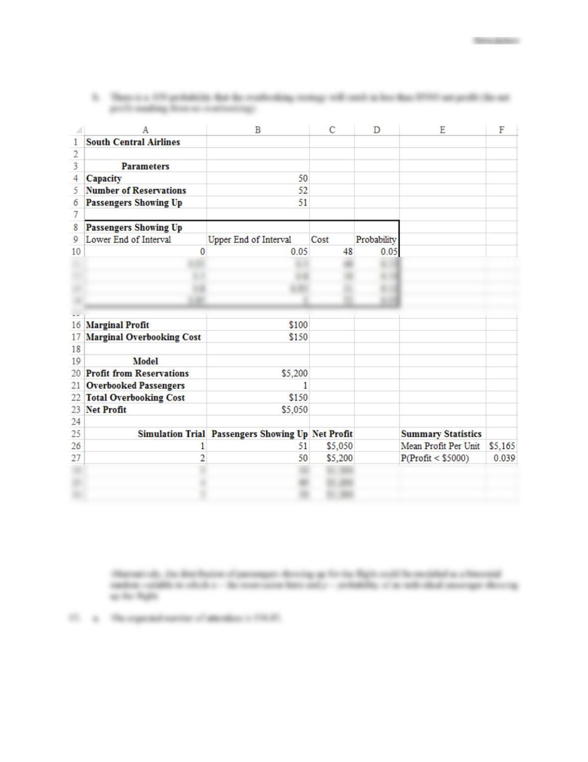
12. a. Average net profit is $5,165.
c. The same spreadsheet design can be used to simulate other overbooking strategies including accepting 51,
53 and 54 passenger reservations. In each case, South Central would need to estimate the distribution of
the number of passengers showing up and rerun the simulation model. This would enable South Central
to evaluate the other overbooking alternatives and determine at the most beneficial overbooking policy.
Chapter 16
16 –
14
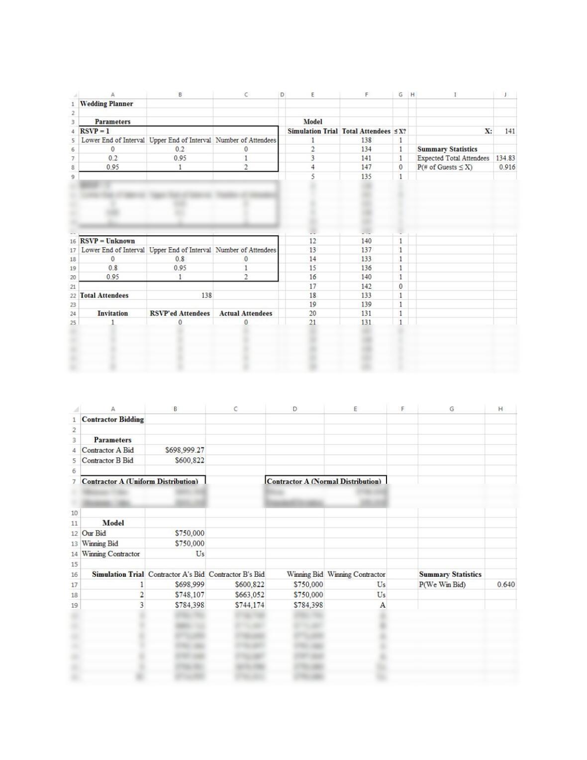
b. P(X ≤ 140) ≈ 89.3% and P(X ≤ 141) ≈ 91.6%. So 141 guests would be a relatively safe number on which
to base meal preparations.
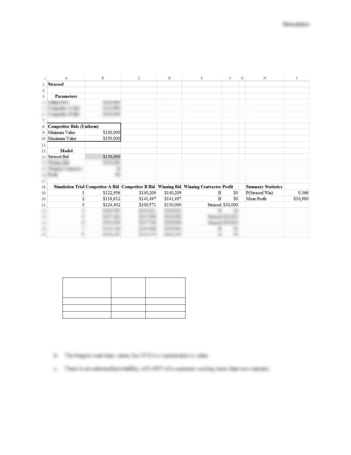
14. a. The building contractor wins the bid about 64% of the time with a bid of $750,000.
16 –
15
b. Bidding $765,000 results in winning approximately 75% of the time. Bidding $775,000 results in winning
approximately 82% of the time. Thus, to assure at least an 80% of winning the bid, we must bid $775,000.
15. a. If Strassel bids $130,000, it has approximately a 36.6% chance of winning the property.
b. To guarantee winning the property, Strassel must bid have a probability of 1.0 that it will have the largest
bid. This will occur if Strassel bids $150,000 which results in $160,000 – $150,000 = $10,000 profit.
c. A bid of $140,000 results in the largest mean profit of the three alternatives.
Bid
Probability
of Winning
Property
Mean Profit
$130,000
0.366
$10,980
$140,000
0.630
$12,600
$150,000
1.000
$10,000
16. Estimates possess non-neglible variability.
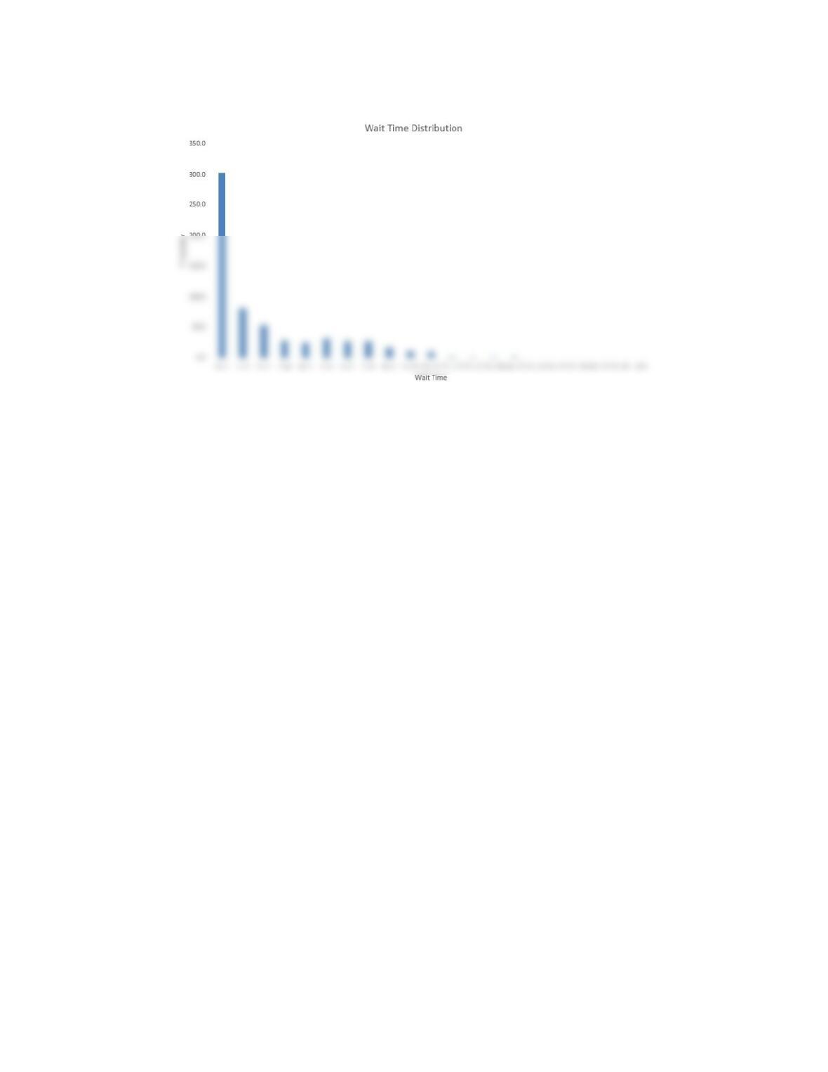
a. Average wait time is approximately 2.29 minutes.
Chapter 16
16 –
16
d.
e. It is not appropriate to increase the number of trials because Burger Dome is trying to model the waiting
line behavior during its 14-hour work day. Assuming that the store opens empty every day (no customers
left over from previous day), this means that the simulation model must correspond to the same amount of
time as the work day.
Simulation
16 –
17
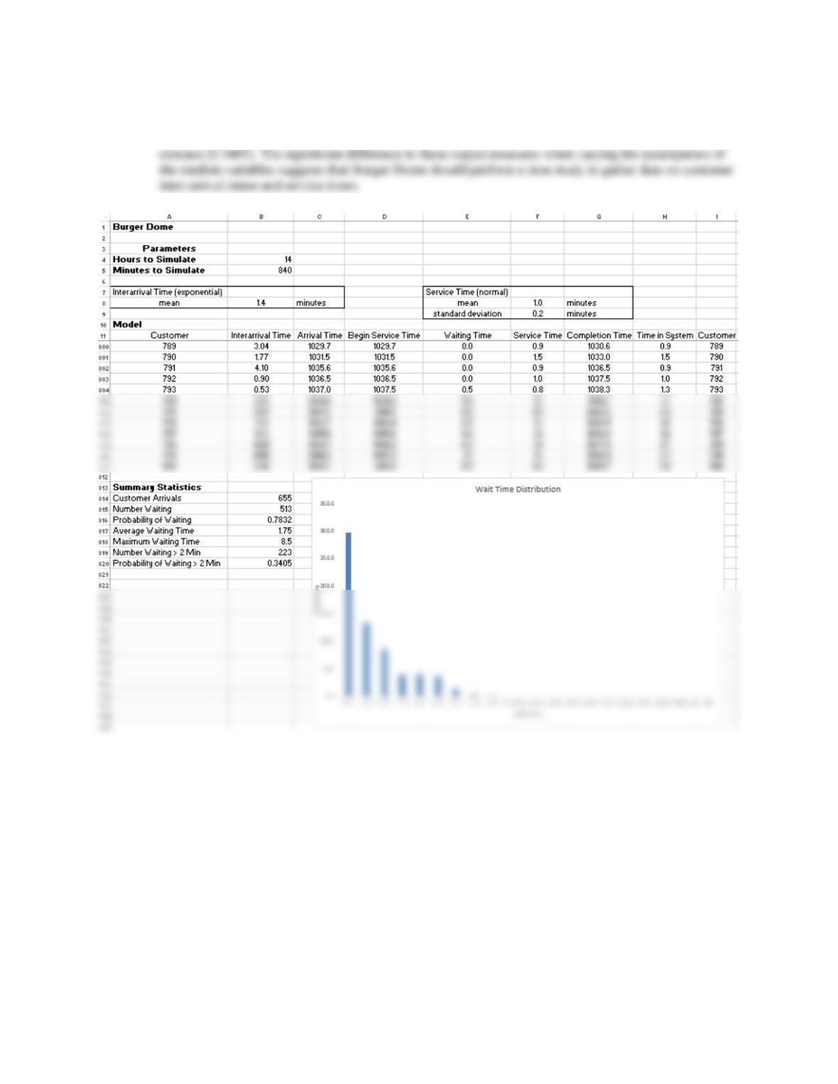
17. Estimates possess non-neglible variability, but modeling service time as a normal random variable with
mean = 1.0 minute and standard deviation = 0.2 minutes results in a reduced average wait time (1.75
minutes), decreased maximum wait time (8.5 minutes), and decreased probability of waiting more than 2
Chapter 16
16 –
18
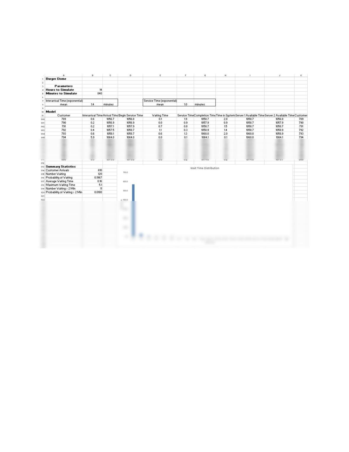
18. Estimates possess considerable variability, but adding a second employee results in a reduced average
wait time (0.16 minutes), decreased maximum wait time (5.1 minutes), and decreased probability of
waiting more than 2 minutes (0.0180). Burger Dome needs to evaluate whether these improvements are
worth the cost of the second employee.
16 –
19
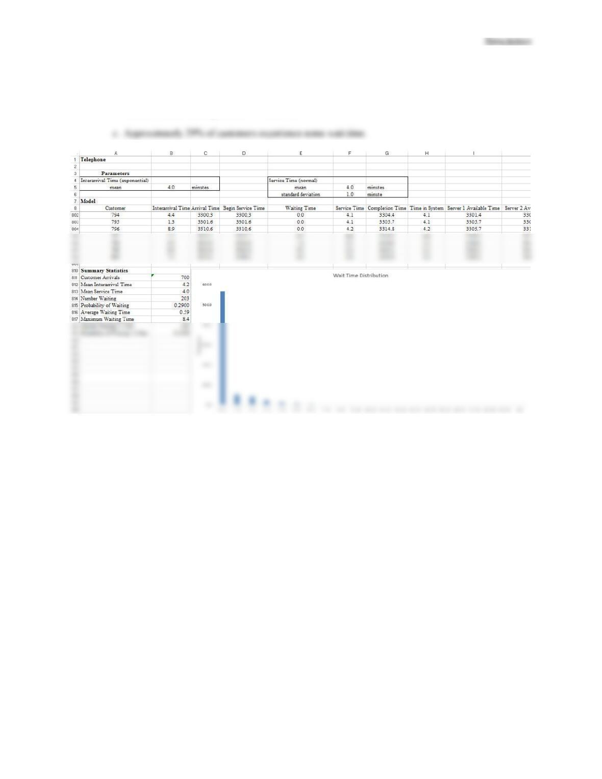
19. a. The mean interarrival time of 4.2 and mean service time of 4.0 suggest that the simulation model is
operation correctly.
b. Mean customer waiting time is 0.59 minutes.
Chapter 16
16 –
20
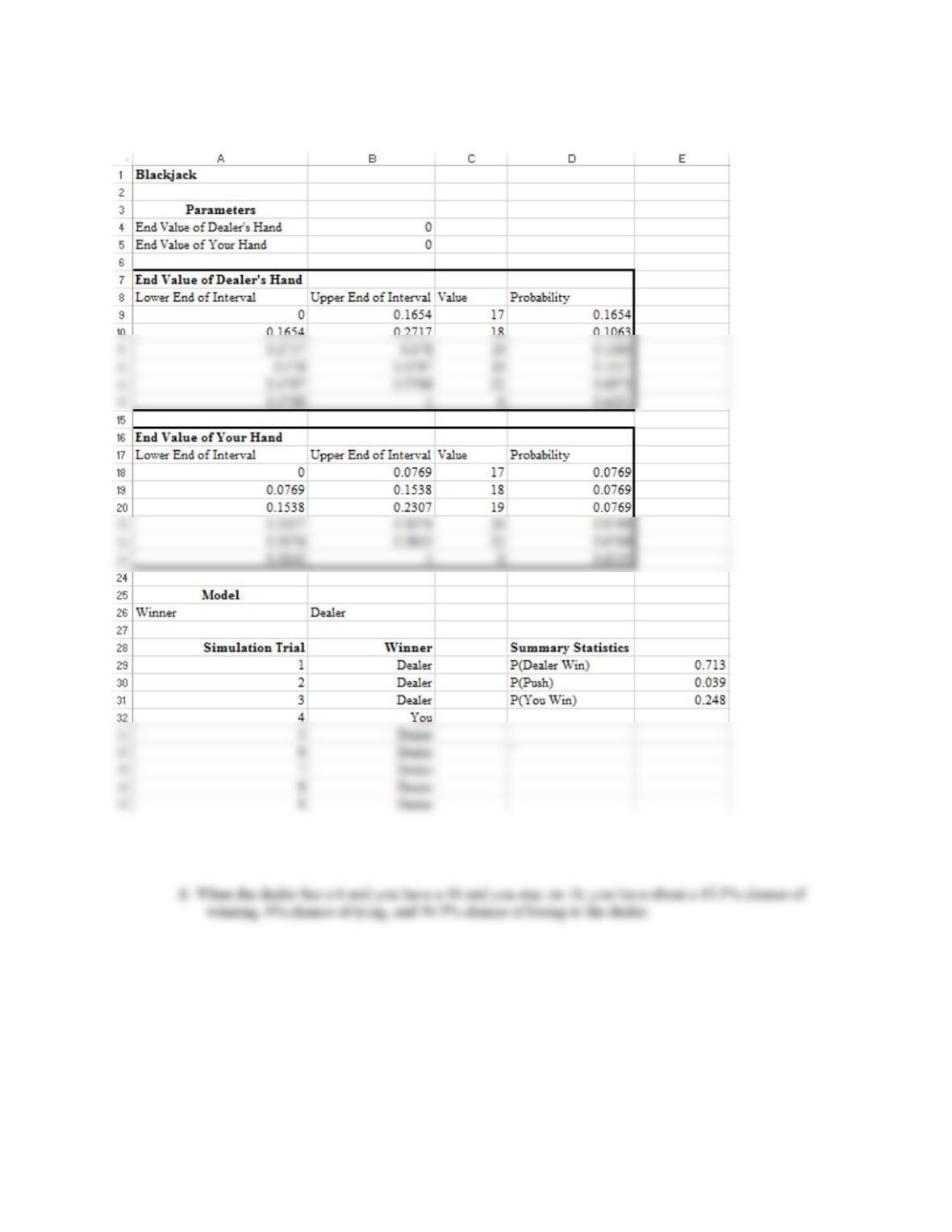
20. a, b. See the figure below.
c. When the dealer has a 6 and you have a 16 and you decide to hit, you have about a 24.8% chance of
winning, 3.9% chance of tying, and 71.3% chance of losing to the dealer.