
Chapter 16 – Scheduling
16-1
CHAPTER 16
SCHEDULING
Teaching Notes
Scheduling techniques are designed to disaggregate the master production schedule into time-phased daily
or hourly activities. A detailed production schedule must include when and where each activity must take
place in order to meet the master schedule.
Scheduling involves the following major activities:
2. Short-run capacity planning.
4. Dispatching (issuing the order to begin work).
6. Controlling the progress of orders and monitoring the process to determine that operations are
running according to plan.
8. Revising the schedule based on changes in order status of jobs, material and/or capacity
availability and various other reasons.
Elements of Scheduling Problems:
1. Job arrival patterns (static vs. dynamic). Dynamic arrival pattern means that more jobs will arrive
2. Ratio of workers to machines (machine limited vs. labor limited environment).
4. Flow patterns of jobs through the plant.
a. Flow shop: All jobs follow the same pattern of flow through the system. In a flow shop,
5. Evaluation of the scheduling technique (maximization of service level, minimization of stockouts,
6. Number and types of machines in the plant (as the number and types of machines increase, the
scheduling environment gets more complicated.)
Chapter 16 – Scheduling
Scheduling decision is based on the following critical factors:
1. Material availability.
3. Bottleneck vs. nonbottleneck operations.
5. Queue of work before each work station.
A major portion of the chapter is devoted to production scheduling. I generally emphasize production
scheduling because it has more “meat” than other areas of scheduling and because it enables students to
get a better grasp on what scheduling involves and some of the tools available.
Answers to Discussion and Review Questions
1. Job shops are intended to handle a wide range of processing requirements; jobs tend to follow
many different paths through the shop, and often differ significantly with respect to processing
2. The main decision areas of job shop scheduling concern loading and sequencing.
3. Gantt charts are visual aids used by managers to plan and adjust facility and equipment loading.
Advantages of Gantt charts include ease of manipulation, the fact that they provide a visual model
4. The assignment model assumes a one-for-one matching is possible, that costs for each
5. a. FCFS: process jobs in order of arrival.
b. SPT: process jobs according to processing times, shortest ones first.
6. Priority rules allow for the fact that jobs are not equally important: different processing sequences

Chapter 16 – Scheduling
16-3
7. Service systems must usually contend with random arrivals and variations in service times.
8. Forward scheduling is when scheduling starts with a specific date and moves forward;
9. To the extent that scheduling efforts can achieve a balance in facility or equipment loading, the
10. Will throughput time decrease? Is it technically feasible to split a job? How disruptive will it be?
What additional costs will be involved (e.g., setup, increased paperwork)?
11. Makespan is the total time needed to complete a group of jobs from the beginning of the first job
to the completion of the last job.
Taking Stock
1. In sequencing jobs, we have to consider the trade-off between the customer service and
operational efficiency. Sequencing job A before job B may result in higher customer service,
because we could meet the due dates of both jobs, but this sequence may be inefficient due to the
2. In large facilities, Production Planning and Control manager, or planners and schedulers are
3. Technology, more specifically, the computers had a profound impact on scheduling. When the
schedule is determined, it can be automatically released from manufacturing control to the shop
Critical Thinking Exercise
1.
a. The production bottleneck limits the production of the entire system due to insufficient
Chapter 16 – Scheduling
16-4
c. If we use small lot sizes for the purpose of reducing the bottleneck effect, it will cost us
more due to more frequent setups, because we will have to produce additional batches.
On the other hand, smaller lot sizes will result in less work-in process inventory and
smaller transfer batches, which in turn will increase the throughput of the system.
2. Unless each customer or job is expected to have the same processing time requirements,
scheduling at regular intervals will tend to create waiting lines. Ideally, appointments should be
3. Student answers will vary.

Chapter 16 – Scheduling
16-5
Memo Writing Exercises
1. Job-shop scheduling is used in producing make-to–order products. These products are usually
made in small batches, they have a wide variety of processing and setup requirements, material
needs and processing sequences. The characteristics listed above make job shop scheduling very
complex and difficult. None of these characteristics are present in the call-in service phone line.
2. The local approach to scheduling only considers the criteria and scheduling issues at a given
workstation (department) without considering the priorities and scheduling issues at other
Chapter 16 – Scheduling
16-6
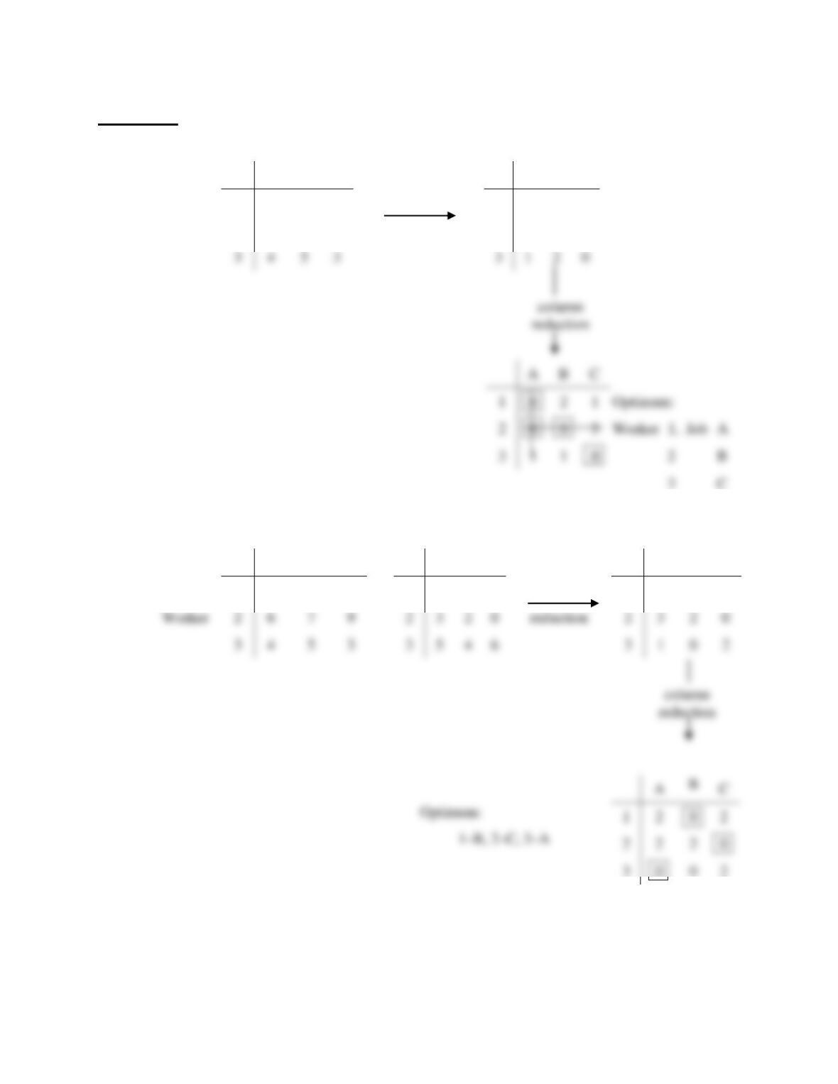
Solutions:
1.
Job
A
B
C
A
B
C
1
5
8
6
row
1
0
3
1
Worker
2
6
7
9
reduction
2
0
1
3
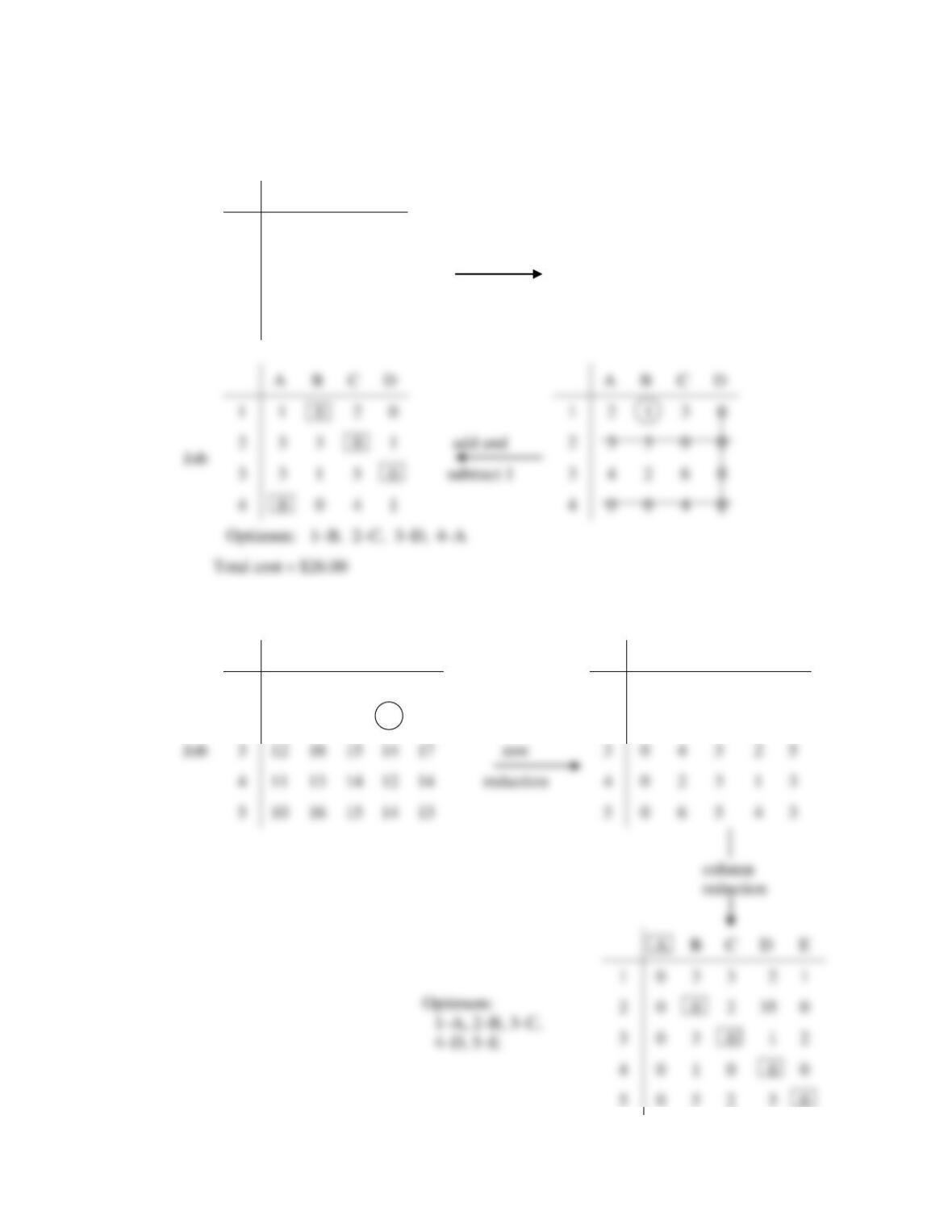
2.
Initial
Job
Initial
revised
A
B
C
A
B
C
A
B
C
1
5
8
6
1
4
1
3
row
1
3
0
2
Worker
2
6
9
2
3
2
3
2
0
3
4
3
3
5
3
1
0
2
1
0
2
0
0
2
3
4
5
3
3
1
2
0
reduction
1
0
2
1
Optimum:
2
0
0
3
Worker
1,
Job
A
3
1
1
0
2
B
3
C
Chapter 16 – Scheduling
16-7
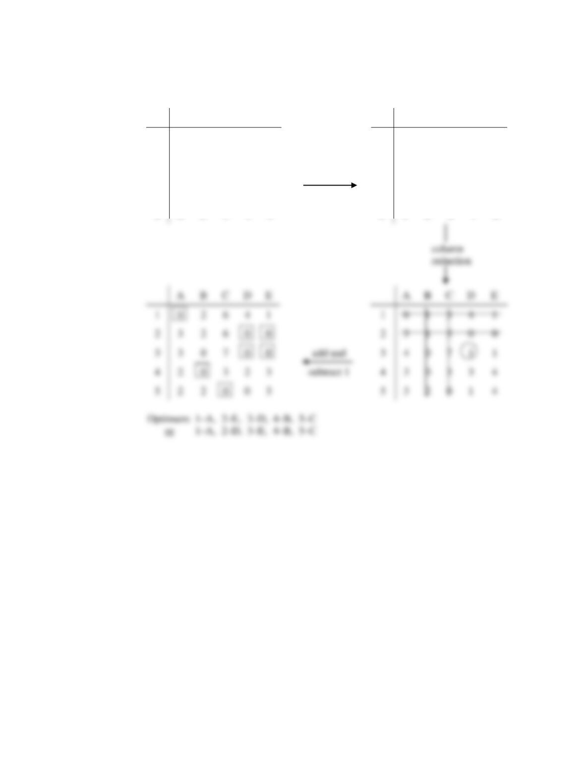
3.
Route
A
B
C
D
E
A
B
C
D
E
1
4
5
9
8
7
1
0
1
5
4
3
2
6
4
8
3
5
2
3
1
5
0
2
Truck
3
7
3
10
4
6
row
3
4
0
7
1
3
4
5
2
5
5
8
reduction
4
3
0
3
3
6
5
6
5
3
4
9
5
3
2
0
1
6
A
B
C
D
E
A
B
C
D
1
0
2
4
2
3
2
6
0
0
3
1
5
0
3
3
0
7
0
0
add and
4
0
7
1
4
2
0
3
2
3
subtract 1
3
0
3
3
Chapter 16 – Scheduling
16-8
4.
Initial + Dummy
Machine
A
B
C
D
1
12
8
11
0
Job
2
13
10
8
0
row
[no change due to dummy]
3
14
9
14
0
reduction
4
10
7
12
0
column
reduction
5.
a. Initial revised
Machine
A
B
C
D
E
A
B
C
D
E
1
14
18
20
17
18
1
0
4
6
3
4
2
14
15
19
50
17
2
0
1
5
36
3
3
12
16
15
14
17
row
3
0
4
3
2
5
4
11
13
14
12
14
reduction
4
0
2
3
1
3
5
10
16
15
14
13
5
0
6
5
4
3
A
B
C
D
2
1
0
0
2
35
0
0
3
0
1
2
A
B
C
D
A
B
C
D
1
1
0
2
0
1
2
1
3
0
Job
2
3
3
0
1
add and
2
3
3
0
0
3
3
1
5
0
subtract 1
3
4
2
6
0
4
0
0
4
1
4
0
0
4
0
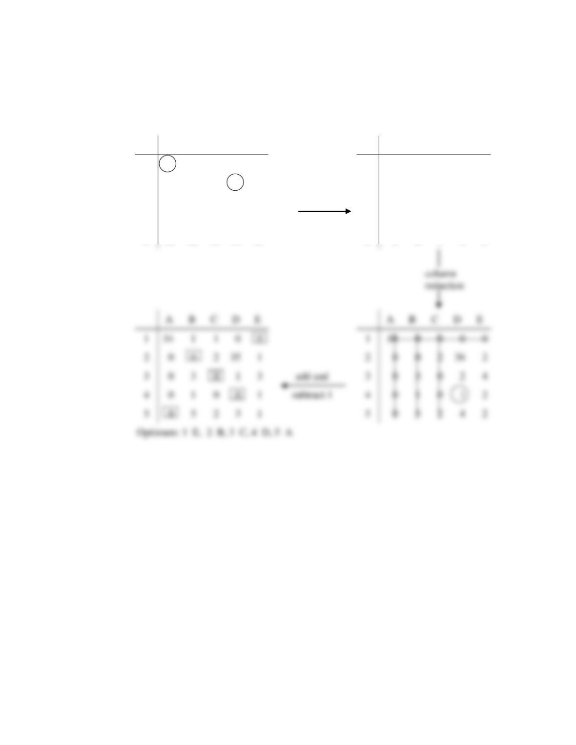
Optimum:
Chapter 16 – Scheduling
16-9
5.
b. Initial revised
Machine
A
B
C
D
E
A
B
C
D
E
1
50
18
20
17
18
1
33
1
3
0
1
2
14
15
19
50
17
2
0
1
5
36
3
Job
3
12
16
15
14
17
row
3
0
4
3
2
5
4
11
13
14
12
14
reduction
4
0
2
3
1
3
5
10
16
15
14
13
5
0
6
3
4
3
A
B
C
D
E
A
B
C
D
E
1
1
38
0
0
0
0
2
2
0
0
2
36
2
3
add and
3
0
3
0
2
4
4
subtract 1
4
0
1
0
1
2
5
5
0
5
2
4
2
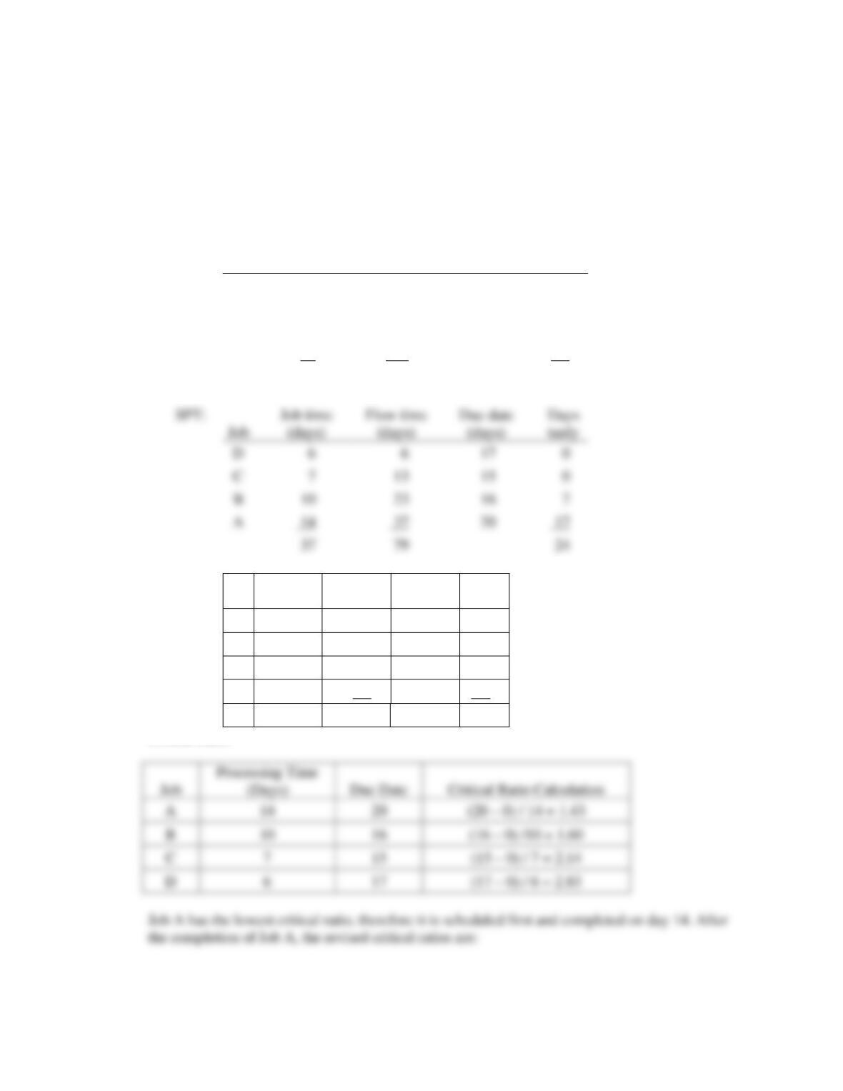
Optimum: 1–E, 2–B, 3–C, 4–D, 5–A
Chapter 16 – Scheduling
16–10
6.
a.
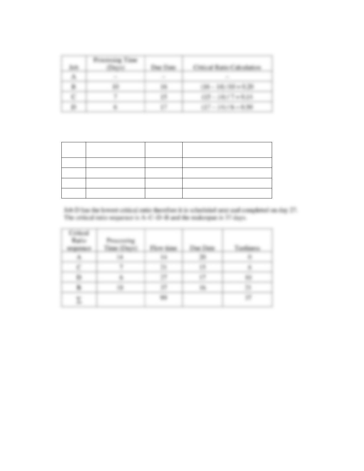
FCFS: A–B–C–D
SPT: D–C–B–A
EDD: C–B–D–A
CR: A–C–D–B
FCFS:
Job time
Flow time
Due date
Days
Job
(days)
(days)
(days)
tardy
A
14
14
20
0
B
10
24
16
8
C
7
31
15
16
D
6
37
17
20
37
106
44
EDD:
Job time
Flow time
Due date
Days
Job
(days)
(days)
(days)
tardy
C
7
7
15
0
B
10
17
16
1
D
6
23
17
6
A
14
37
20
17
84
24
Critical Ratio
C
Job time
Flow time
Due date
Days
Job
(days)
(days)
(days)
tardy
D
6
17
0
C
13
15
0
B
10
23
16
7
A
14
37
20
17
37
79
Chapter 16 – Scheduling
16–11
Job C has the lowest critical ratio, therefore it is scheduled next and completed on day 21. After
the completion of Job C, the revised critical ratios are:
Job
Processing Time
(Days)
Due Date
Critical Ratio Calculation
A
–
–
–
B
10
16
(16 – 21) /10 = –0.50
C
–
–
–
D
6
17
(17 – 21) / 6 = –0.67
A
14
20
C
21
D
27
B
37
A
B
10
16
C
15
D
17

Chapter 16 – Scheduling
16–12
jobs 67.2
37
99
jobs of number Average
==
b.
jobs of Number
time Flow
time flow Average
=
FCFS
SPT
EDD
CR
26.50
19.75
21.00
24.75
Chapter 16 – Scheduling
16–13
7.
FCFS: a–b–c–d–e
SPT: c–b–a–e–d
EDD: a–b–c–e–d
CR: a–e–b–c–d
FCFS:
Operation
Flow time
Due date
Hours
Job
time (hr.)
(hr.)
(hr.)
tardy
a
7
7
4
3
SPT:
Operation
Flow time
Due date
Hours
Job
time (hr.)
(hr.)
(hr.)
tardy
c
2
2
12
0
b
4
6
10
0
a
7
13
4
9
e
8
21
15
6
32
74
EDD:
Operation
Flow time
Due date
Hours
Job
time (hr.)
(hr.)
(hr.)
tardy
a
7
7
4
3
b
4
11
10
1
c
2
13
12
1
e
8
21
15
6
d
20
32
84
b
4
10
1
c
2
13
12
1
d
11
24
20
4
e
15
32
87
Chapter 16 – Scheduling
16–14
Critical Ratio
Job
Processing Time
(Hours)
Due Date
Critical Ratio Calculation
A
(.14 x 45) + .7 = 7
4
(4 – 0) / 7 = .57
B
(.25 x 14) + .5 = 4
10
(10 – 0) / 4 = 2.5
Job A has the lowest critical ratio, therefore it is scheduled first and completed after 4 hours, the
revised critical ratios are:
Job
Processing
Time (Hrs.)
Due Date
Critical Ratio Calculation
A
–
–
–
C
D
E
Job B has the lowest critical ratio therefore it is scheduled next and it is completed after 11 hours
(7 + 4). After the completion of Job B, the revised critical ratios are:
Job
Processing Time
(Hours)
Due Date
Critical Ratio Calculation
A
–
–
–
B
–
–
–
D
D
Chapter 16 – Scheduling
16–15
Job
Processing Time
(Hours)
Due Date
Critical Ratio Calculation
A
–
–
–
B
–
–
Job E has the lowest critical ratio therefore it is scheduled next. The critical ratio final sequence is
A–B–C–E–D. Total completion of all six jobs (makespan) is 32 hours.
Critical Ratio
sequence
Processing
Time (Days)
Flow time
Due Date
Tardiness
A
7
7
4
3
B
4
11
10
1
C
2
13
12
1
E
8
21
15
6
D
32
20
jobs of Number
time Flow
time flow Average
=
FCFS
SPT
EDD
CR
17.40
14.80
16.80
16.8
C
–
–
20
E
15
Chapter 16 – Scheduling
16–16
8.
a.
(1) FCFS: A–B–C–D–E
(2) S/O: B–D–C–A–E OR D–B–C–A–E [see below]
Time
Due date
Remaining number
Job
(days)
(days)
Slack
of operations
Ratio
Rank
A
8
20
12
2
6.0
4
b. S/O: [Assume B–D–C–A–E]
Time
Flow time
Due date
Days
Job
(days)
(days)
(days)
tardy
B
10
10
18
0
D
11
21
17
4
C
5
26
25
1
A
8
34
20
14
E
9
35
8
43
134
27
Time
Flow time
Due date
Days
Job
(days)
(days)
(days)
tardy
A
8
8
20
0
B
10
18
18
0
C
5
23
25
0
D
11
34
17
17
E
9
35
43
126
25
S/O
flow time:
B
10
18
8
4
2.0
C
5
25
20
5
4.0
3
D
11
17
6
3
2.0
E
9
35
26
4
6.5
5
Chapter 16 – Scheduling
16–17
9.
Time (hr.)
Order
Step 1
Step 2
B
0.90
1.30
C
2.00
0.80
D
1.70
1.50
1.60
1.80
F
2.20
1.75
G
1.30
1.40
Sequence of assignment:
.80
[C]
last (i.e., 7th)
.90
[B]
first
1.20
[A]
2nd
1.30
[G]
3rd
1.60
[E]
4th
1.50
[D]
6th
1.75
[F]
5th
A
1.20
1.40
Chapter 16 – Scheduling
16–18
10.
a.
Job
Machine A
Machine B
a
16
5
7
b
3
2
13
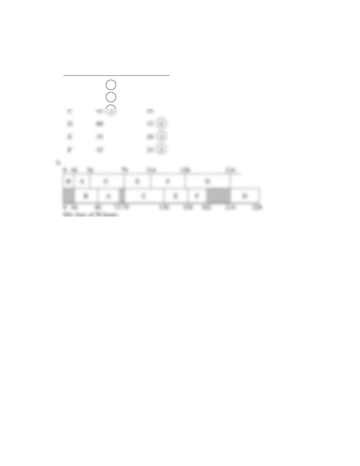
Thus, the sequence is e–b–g–h–d–c–a–f.
c
9
6
6
b.
0 2 5 23 43 51 60 76 88
e
B
g
h
d
c
a
f
e
b
g
h
d
c
After splitting, we get the following Gantt chart:
0 2 5 23 43 51 60 68 76 82 88
e
b
g
h
d
c
a1
a2
f1
f2
e
b
g
h
d
c
a1
a2
f1
f2
0 2 16 29 43 54 61 67 68 70.5 76 78.5 84 90
d
8
7
5
e
2
1
14
4
8
g
18
14
3
h
20
11
4
Chapter 16 – Scheduling
16–19
Time (minutes)
11.
a.
Job
Center 1
Center 2
A
20
2
27
B
16
1
30
Thus, the sequence is B–A–C–E–F–D.
C
43
3
51
D
60
12
6
E
35
28
4
42
24
5
b.
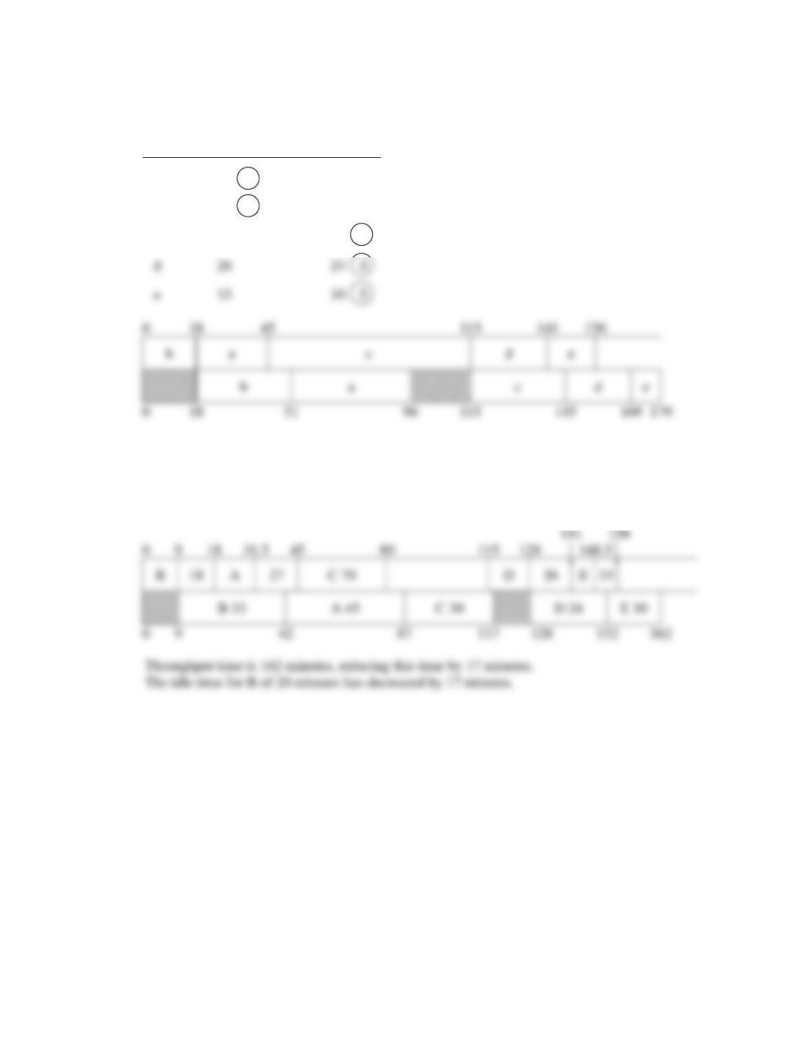
Chapter 16 – Scheduling
16–20
12.
a.
Job
Station A
Station B
a
27
2
45
b
18
1
33
Thus, the sequence is b–a–c–d–e.
c
70
30
3
b.
The Idle time for Station B is = 18 + 19 = 37 minutes.
c.
Jobs B, A, C, D and E are candidates for splitting in order to reduce throughput time and idle
time.
d
26
24
4
e
15
10
5