Excel Templates to accompany Operations Management, Eleventh Edition
created by Lee Tangedahl
Copyright © 2012 by The McGraw Hill Companies, Inc. All rights reserved.
Chapter Sixteen – Scheduling
Templates: Assignment Model (Basic) Solved Problems: Solved Problem 1
Job Sequencing Solved Problem 2,3
Johnson’s Rule Solved Problem 4
Cyclical Scheduling Solved Problem 5
See the Transportation Model tutorial for a demonstration of the transportation model (similar to the Assignment Model).
See Instructions template for complete instructions.
Lecture Suggestions Problems: Problems 1-8
Example 2
Example 3
Example 4
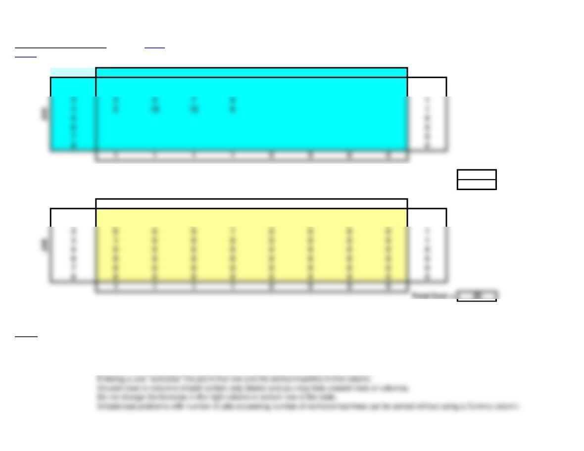
Assignment Model (Basic) Notes Use Solver on Data Ribbon to solve – see notes below.
<Back
Input Matrix: Worker/Machine
A B C D E F G H
1 8 6 2 4 1
2 6 7 11 10 1
Total Jobs = 4
Do not change or delete unshaded cells. Total Workers/Machines = 4
Solution Matrix: Worker/Machine
A B C D E F G H
1 0 0 1 0 0 0 0 0 1
2 0 1 0 0 0 0 0 0 1
4 1 0 0 0 0 0 0 0 1
5 0 0 0 0 0 0 0 0 0
6 0 0 0 0 0 0 0 0 0
7 0 0 0 0 0 0 0 0 0
Notes: See the Transportation Model tutorial for a demonstration of the transportation model (similar to this template).
1. Enter the problem into the Input Matrix (top shaded area):
Enter the name of the worker/machine in the top row and job name in the left column (optional).
Enter the costs to assign each worker/machine to each job in the middle of the matrix.
3 3 5 7 6 1
Unbalanced problems with number of workers/machines exceeding number of jobs are not feasible and will require a Dummy row.
2.
You can manually create solutions in the Solution Matrix (bottom shaded area):
Enter 1’s to assign workers/machines to jobs in the middle of the Solution Matrix (shaded yellow).
3. Using Solver to find the optimal solution:
Select the Data ribbon, the Solver Add-in must be available in the Analysis group (see note below to add-in Solver).
More… 4. Notes on the Solver solution:
Small numbers in scientific notation (e.g. 2.4091E-11) reflect the precision of Solver and can be treated as zero.
5. How to Add-In Solver if it does not appear in the Analysis group of the Data ribbon:
Select File (left-most item in main menu at top of screen).
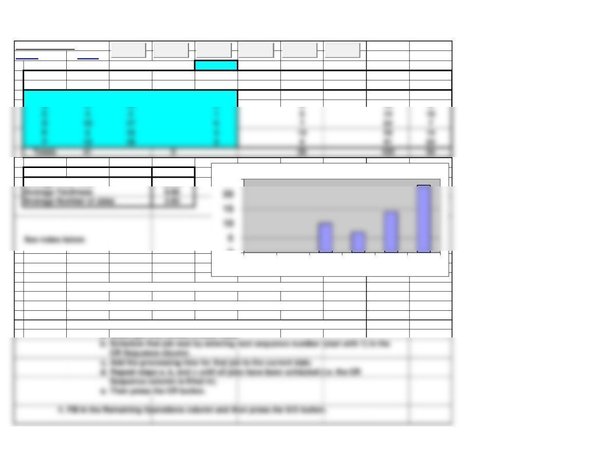
Job Sequencing
Job Sequencing
<Back Notes
Current Date: 23
Process. Due Remain CR Critical Flow Days
Job Time Date Oper. Sequence Ratio Slack S/O Time Late
A 2 7 3 5 2 0
Method FCFS
Average Flow Time 20.00 A 0
Average Tardiness 9.00 B 0
Notes:
1. Enter Job Name, Processing Time, and Due Date for each job.
2.
For the FCFS, SPT, and DD rules, simply press the appropriate button.
3. For the CR rule, perform the following BEFORE pressing the CR button:
a. Select job with lowest Critical Ratio
4. Fill in the Remaining Operations column and then press the S/O button.
0
25
A B C D E F
Days Late
Clear
FCFS
SPT
DD
CR
S/O
Page 4

Job Sequencing
Back to top
Page 5
Johnson’s Rule
Johnson’s Rule
<Back
Step 1 – Fill in jobs and times: Resulting schedule:
Job Time1 Time2 Job Start 1 Done 1 Start 2 Done 2 Idle 2
A 5 5 D 0 2 2 9 2
B 4 3 E 2 8 9 17 0
Step 2 – Assign job order:
A D E C F A B
B
C
D
E
Clear
Cyclical Scheduling
Cyclical Scheduling
<Back
Mon Tue Wed Thu Fri Sat Sun
Staff Needed 2 4 3 4 6 5 5
Unmet Need 0 0 0 0 0 0 0
Worker 1 w w w w w 5
Worker 2 w w w w w 5
Worker 3 w w w w w 5
Worker 4 w w w w w 5
Clear
Page 7
Worker 5 w w w w w 5
Worker 6 w w w 3
Worker 7 w 1
Worker 8 0
Lecture Suggestions – Chapter 16
<Back
Example 2: Scheduling – Critical Ratio method
2. (Optional) Clear worksheet (press Clear and confirm with OK) and re-enter data for Job, Process
Time, and Due Date.
3. Enter Current Date = 0.
4. Point out that Critical Ratio = (Due Date – Current Date) / Process Time are computed for each job.
5. Pick job with lowest critical ratio (Job C) and enter a 1 (first to be done) in the CR sequence column.
6. Add processing time for Job C (4) to current time so Current Time = 4.
7. Point out that that critical ratios are re-computed:
8. Pick job with lowest remaining critical ratio (Job F) and enter a 2 (second to be done) in the CR
9. Add processing time for Job F (12) to current time so Current Time = 16.
Repeat steps 5-6:
10. Pick job with lowest remaining critical ratio (Job A) and enter a 3 (third to be done) in the CR
11. Add processing time for Job A (2) to current time so Current Time = 18.
Repeat steps 5-6:
13. Add processing time for Job E (5) to current time so Current Time = 23.
Repeat step 5:
15. For the only job remaining (Job D) and enter a 6 (last to be done) in the CR sequence column.
16. Press the CR button to sequence jobs.

18. Point out the Days Late for A, B, D, and E in the graph.
17. Compare average flow time, average tardiness, and average number of jobs with other
Assignment Model (Basic) Notes Use Solver on Data Ribbon to solve – see notes below.
<Back
Input Matrix: Worker/Machine
A B C D E F G H
1 8 6 2 4 1
2 6 7 11 10 1
3 3 5 7 6 1
Total Jobs = 4
Do not change or delete unshaded cells. Total Workers/Machines = 4
Solution Matrix: Worker/Machine
A B C D E F G H
1 0 0 1 0 0 0 0 0 1
2 0 1 0 0 0 0 0 0 1
4 1 0 0 0 0 0 0 0 1
5 0 0 0 0 0 0 0 0 0
6 0 0 0 0 0 0 0 0 0
7 0 0 0 0 0 0 0 0 0
Notes: See the Transportation Model tutorial for a demonstration of the transportation model (similar to this template).
1. Enter the problem into the Input Matrix (top shaded area):
Enter the name of the worker/machine in the top row and job name in the left column (optional).
Unbalanced problems with number of workers/machines exceeding number of jobs are not feasible and will require a Dummy row.
2.
You can manually create solutions in the Solution Matrix (bottom shaded area):
Enter 1’s to assign workers/machines to jobs in the middle of the Solution Matrix (shaded yellow).
3. Using Solver to find the optimal solution:
Select the Data ribbon, the Solver Add-in must be available in the Analysis group (see note below to add-in Solver).
More… 4. Notes on the Solver solution:
Small numbers in scientific notation (e.g. 2.4091E-11) reflect the precision of Solver and can be treated as zero.
5. How to Add-In Solver if it does not appear in the Analysis group of the Data ribbon:
Select File (left-most item in main menu at top of screen).
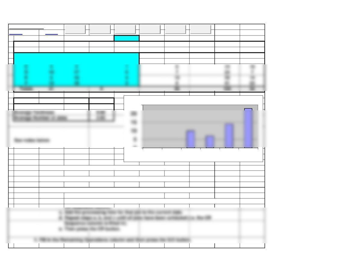
Example 2
Job Sequencing
<Back Notes
Current Date: 23
Process. Due Remain CR Critical Flow Days
Job Time Date Oper. Sequence Ratio Slack S/O Time Late
A 2 7 3 5 2 0
B 8 16 5 8 10 0
Method FCFS
Average Flow Time 20.00 A 0
Average Tardiness 9.00 B 0
Notes:
1. Enter Job Name, Processing Time, and Due Date for each job.
2.
For the FCFS, SPT, and DD rules, simply press the appropriate button.
3. For the CR rule, perform the following BEFORE pressing the CR button:
a. Select job with lowest Critical Ratio
b. Schedule that job next by entering next sequence number (start with 1) in the
c. Add the processing time for that job to the current date.
d. Repeat steps a, b, and c until all jobs have been schduled (i.e. the CR
e. Then press the CR button.
4. Fill in the Remaining Operations column and then press the S/O button.
0
25
A B C D E F
Days Late
Clear
FCFS
SPT
DD
CR
S/O
Page 12

Example 2
Back to top
Page 13
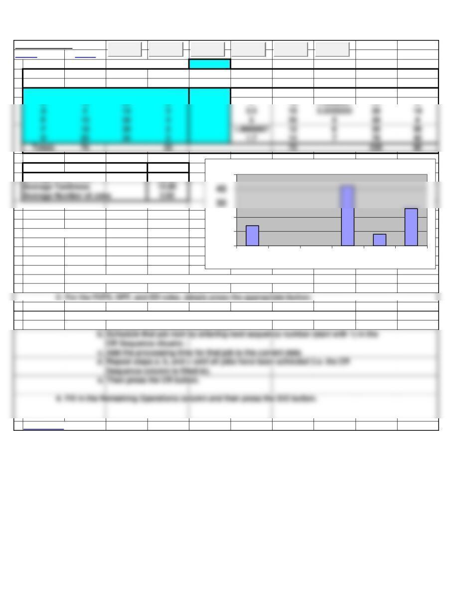
Example 3
Job Sequencing
<Back Notes
Current Date: 0
Process. Due Remain CR Critical Flow Days
Job Time Date Oper. Sequence Ratio Slack S/O Time Late
C 8 8 5 10 0 8 0
Method S/O
Average Flow Time 38.33 A14
Average Tardiness 15.00 B 0
E 8
F26
See notes below.
Notes:
1. Enter Job Name, Processing Time, and Due Date for each job.
2.
For the FCFS, SPT, and DD rules, simply press the appropriate button.
3. For the CR rule, perform the following BEFORE pressing the CR button:
a. Select job with lowest Critical Ratio
c. Add the processing time for that job to the current date.
e. Then press the CR button.
4. Fill in the Remaining Operations column and then press the S/O button.
Back to top
0
10
20
50
A B C D E F
Days Late
Clear
FCFS
SPT
DD
CR
S/O
Page 14
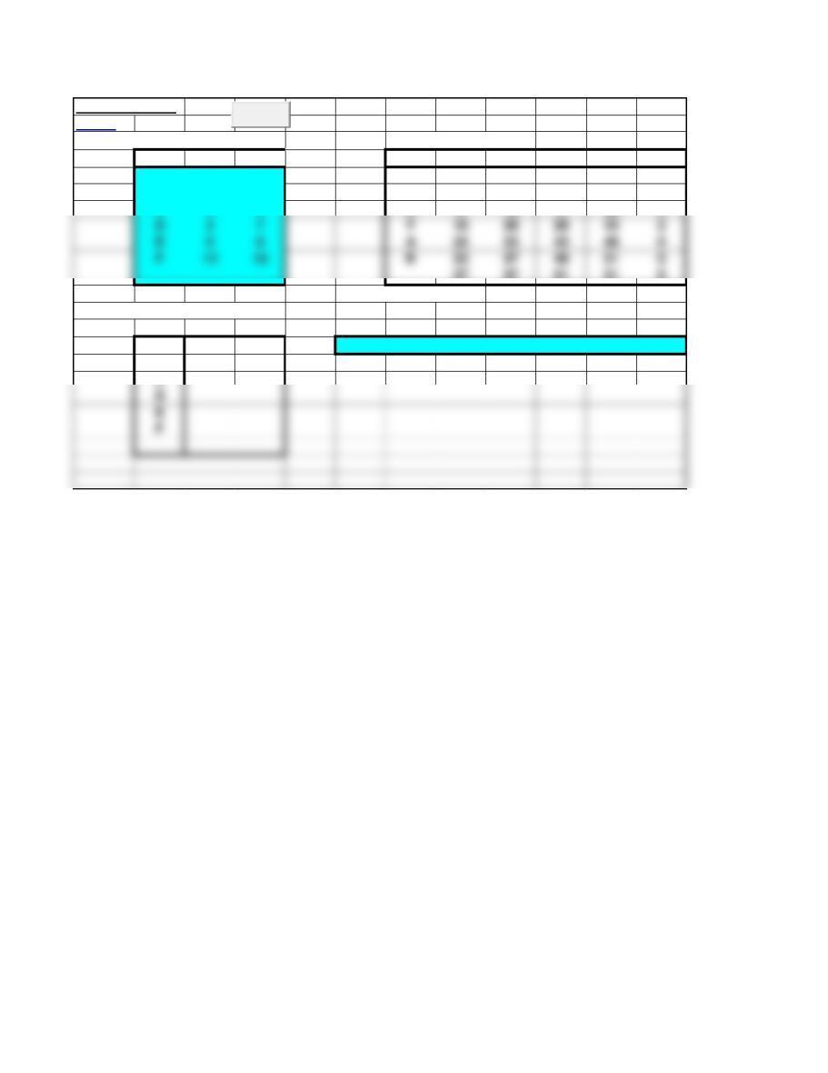
Example 4
Johnson’s Rule
<Back
Step 1 – Fill in jobs and times: Resulting schedule:
Job Time1 Time2 Job Start 1 Done 1 Start 2 Done 2 Idle 2
A 5 5 D 0 2 2 9 2
B 4 3 E 2 8 9 17 0
C 8 9 C 8 16 17 26 0
37 37 51 51 0
Idle time-> 14 4
Step 2 – Assign job order:
A D E C F A B
B
C
D
E
Clear
Page 15
Assignment Model (Basic) Notes Use Solver on Data Ribbon to solve – see notes below.
<Back
Input Matrix: Worker/Machine
A B C D E F G H
112 16 14 10 1
2 9 8 13 7 1
315 12 911 1
Total Jobs = 4
Do not change or delete unshaded cells. Total Workers/Machines = 4
Solution Matrix: Worker/Machine
A B C D E F G H
1 0 0 0 1 0 0 0 0 1
2 0 1 0 0 0 0 0 0 1
3 0 0 1 0 0 0 0 0 1
4 1 0 0 0 0 0 0 0 1
5 0 0 0 0 0 0 0 0 0
6 0 0 0 0 0 0 0 0 0
7 0 0 0 0 0 0 0 0 0
Notes: See the Transportation Model tutorial for a demonstration of the transportation model (similar to this template).
1. Enter the problem into the Input Matrix (top shaded area):
Enter the name of the worker/machine in the top row and job name in the left column (optional).
Unbalanced problems with number of workers/machines exceeding number of jobs are not feasible and will require a Dummy row.
2.
You can manually create solutions in the Solution Matrix (bottom shaded area):
Enter 1’s to assign workers/machines to jobs in the middle of the Solution Matrix (shaded yellow).
3. Using Solver to find the optimal solution:
Select the Data ribbon, the Solver Add-in must be available in the Analysis group (see note below to add-in Solver).
More… 4. Notes on the Solver solution:
Small numbers in scientific notation (e.g. 2.4091E-11) reflect the precision of Solver and can be treated as zero.
If number of workers/machines exceeds number jobs then problem is not feasible and you will get an error message.
5. How to Add-In Solver if it does not appear in the Analysis group of the Data ribbon:
Select File (left-most item in main menu at top of screen).
Select Options (left side of dialog box).