Chapter 16 – Scheduling
16–32
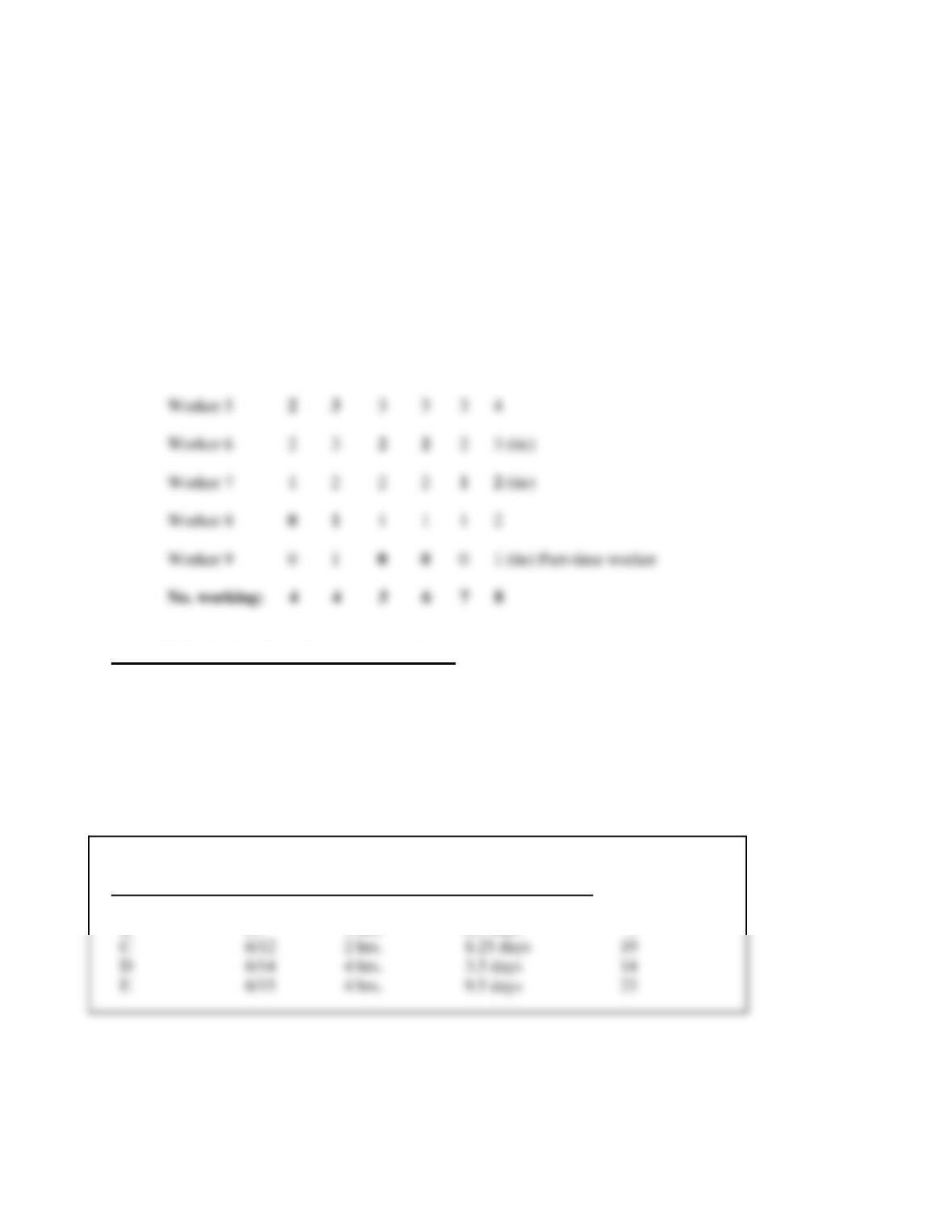
26.
Day Mon Tue Wed Thu Fri Sat
Staff needed 4 4 5 6 7 8
Worker 1 4 4 5 6 7 8
Worker 2 4 4 4 5 6 7 (tie)
Worker 3 3 4 4 4 5 6
Worker 4 3 4 3 3 4 5
Case: Hi-Ho Yo-Yo Case Study Grading Guide
Technical
Did student add setup time to the production time for each order and change due dates to days
From the beginning of schedule?
Date Order Setup Production Due
Job Received Time Time w/ Setup Date
A 6/4 2 hrs. 6.25 days 7
B 6/7 4 hrs. 2.5 days 5
Chapter 16 – Scheduling
16–33
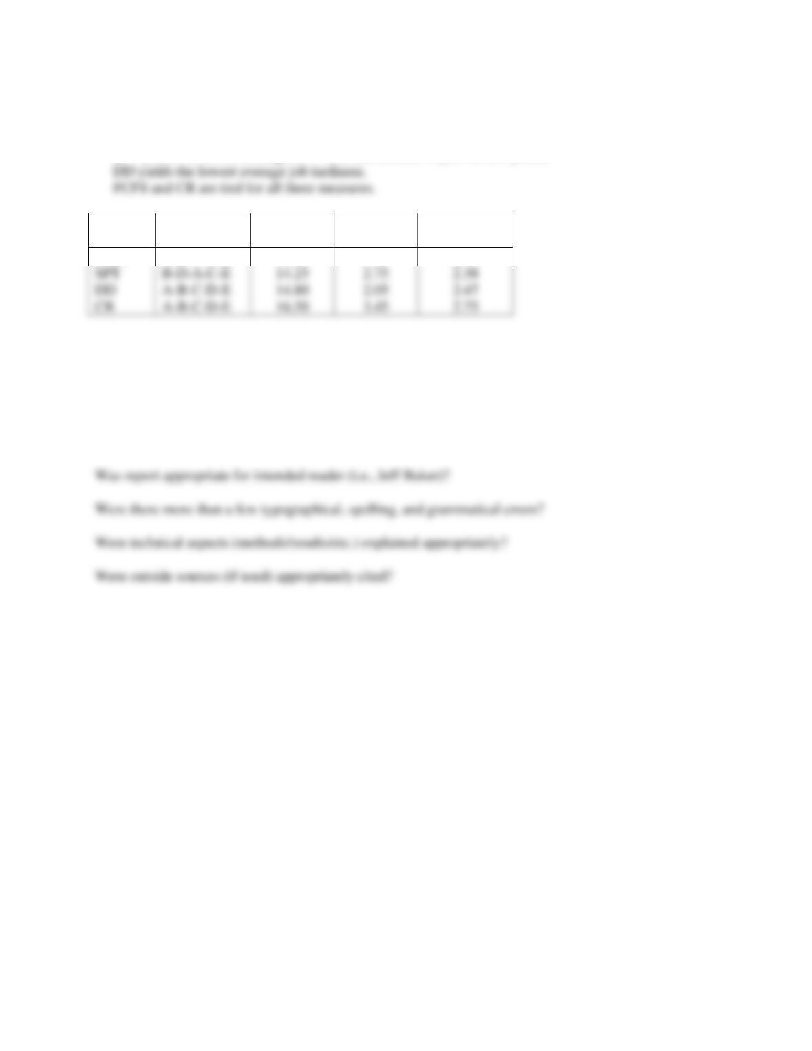
Did the student use all the heuristics available in the templates to evaluate the sequences?
Did the student properly evaluate the results?
SPT yields the lowest average flow time and number of jobs in the system.
Rule
Sequence
Average
flow time
Average
tardiness
Average no.
of jobs late
FCFS
A-B-C-D-E
16.50
3.45
2.75
Did the student discuss tradeoffs, and make and justify a recommendation?
Managerial/Editorial
Was report organized professionally?
Chapter 16 – Scheduling
16–34
Enrichment Module: Runout Time Method
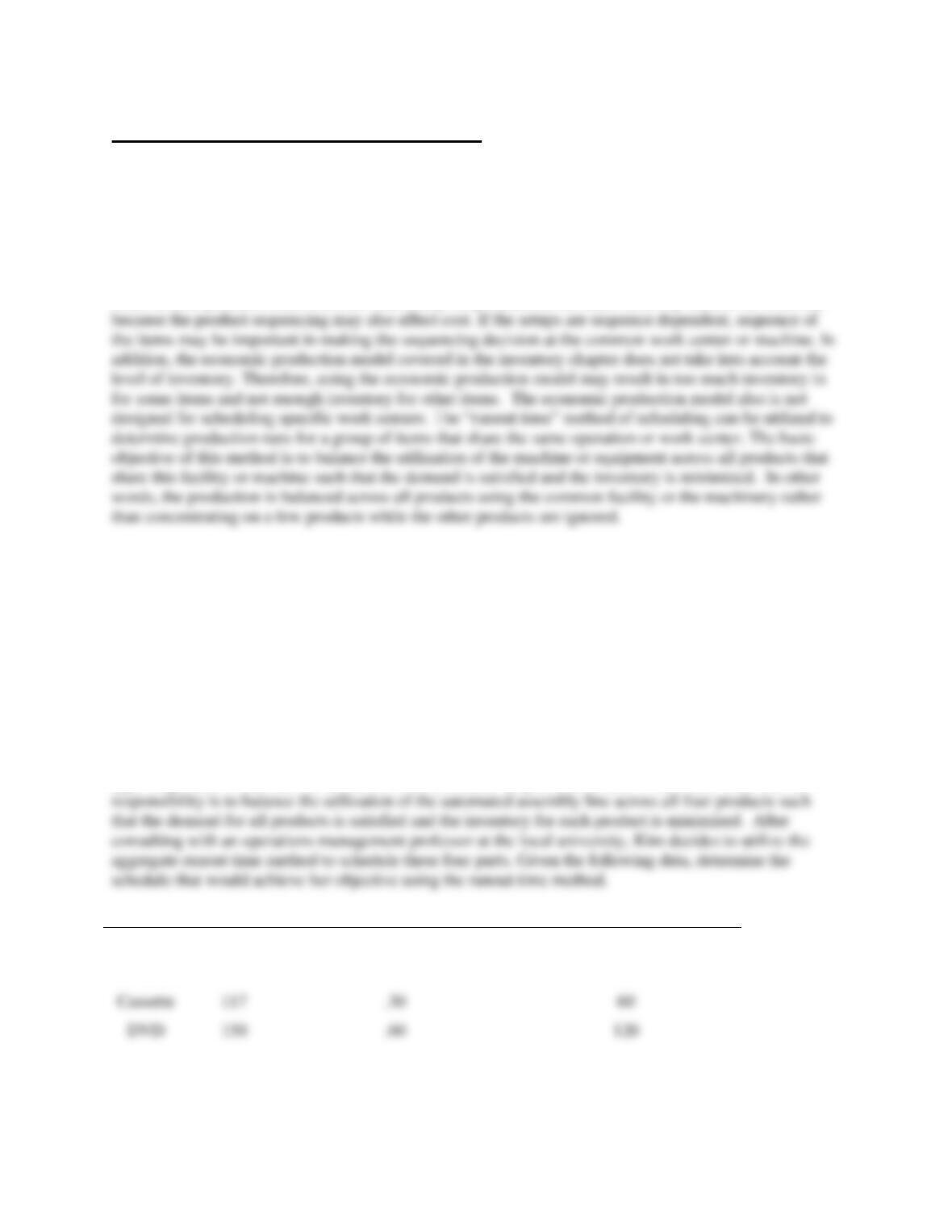
Make-to-stock companies produce different products on a common machine or an operation. For
example, a paint manufacturing company may decide to mix different colors of paint using the same
“mixer”. In this scenario, the plant manager has to decide how much of different colors of paint to
produce in each batch and the sequence of production. This decision is generally made based on the
current level of inventory, production rate associated with a particular product and the rate of demand.
The optimal lot size can be determined using the production lot size model covered in the inventory
management chapter which balances the trade-off between carrying cost and the setup cost. However,
when several products share common machinery for production, the batch sizes my need to be modified
There are two versions of runout method available:
1. Aggregate runout method: This method is used if the lot size is variable.
2. Individual runout time method: This method is used if there are fixed lot sizes.
Aggregate Runout Method
First, we will illustrate the aggregate runout time method with the following example.
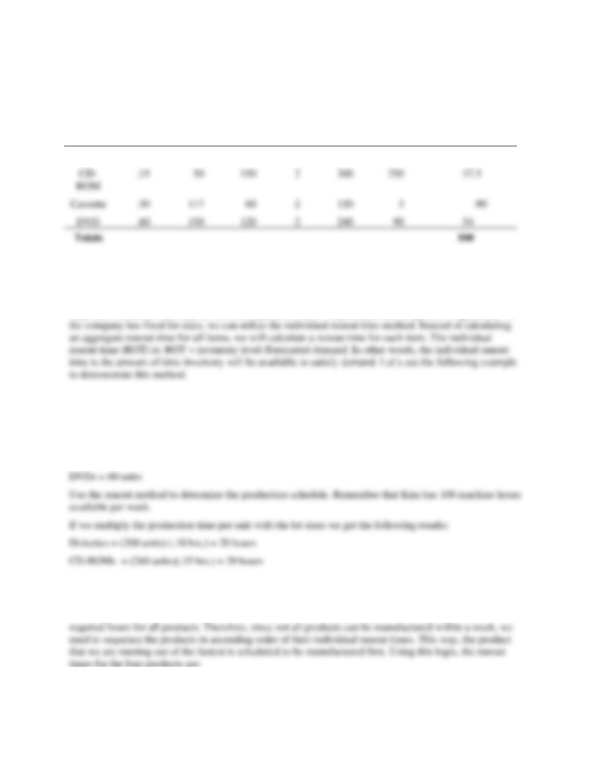
Kim Reuter starts her own company producing computer diskettes, CD-ROMs, DVDs and cassette tapes.
All of these products are processed by the “Blue Monster”, an automated assembly line to produce these
types of products. Kim has 100 machine hours available for production each week. Kim feels that her
Item
Inventory
Production time (hours/unit)
Forecast in units (per week)
Diskette
94
.10
85
CD–ROM
50
.15
150
.60
120
Chapter 16 – Scheduling
16–35
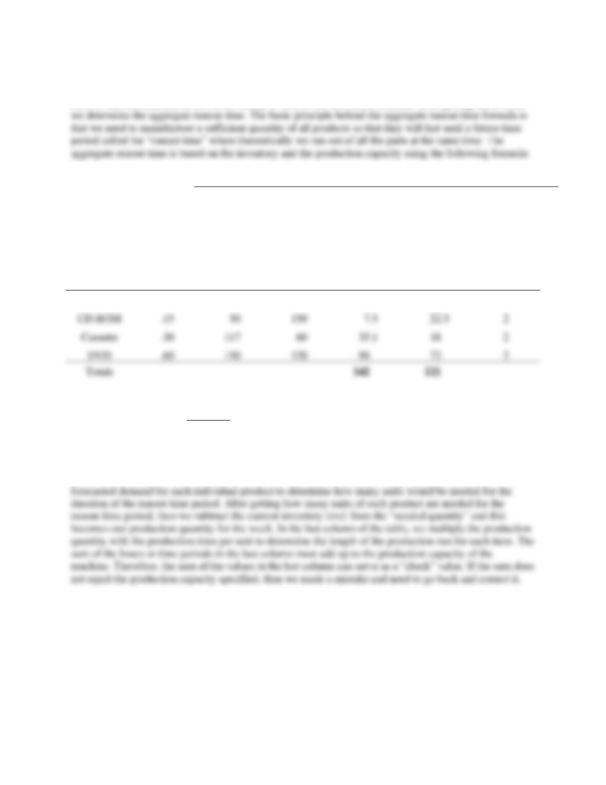
In order to solve this problem, first we must convert all of the inventory and forecasted demand into
machine hours. Once we have the inventory and the forecasted demand in machine hour terms, then we
need to sum the machine hours for inventory as well as the forecasted demand. After getting these totals
Hours Machinein Demand Forecasted Aggregate
Hours Machinein Capacity ProductionHours Machinein Inventory Aggregate
TimeRunout Aggregate +
=
In order to determine the aggregate runout time, we will utilize the following table.
Item
Production
time/unit
(hours)
Inventory
(units)
Forecasted
demand
(units)
Inventory
(hours)
Forecasted
demand
(hours)
Runout time
(in weeks)
Diskette
.10
94
85
9.4
8.5
2
Cassette
.30
60
2
weeks 2
121
100142
erunout tim Aggregate =
+
=
Since the aggregate runout time is two weeks, we need to have two weeks supply of each item, given our
current inventory levels. The following table illustrates the calculation to determine the production
quantities of each item. In these calculations, we start by multiplying the aggregate runout time with
Chapter 16 – Scheduling
16–36
Item
Production
Time
(in hrs.)
(1)
Inventory
(in units)
(2)
Forecast
(in units)
(3)
ROT
(in
weeks)
(4)
# of
items
needed
(5) =
(3)x(4)
Production
schedule
(in units)
(6) =
(5) – (2)
Production
schedule
(in machine hrs).
(7) = (1)x(6)
Diskette
.10
94
85
2
170
76
7.6
Individual Runout Time Method
In many situations, the aggregate runout time method described above is inadequate because the company
produces products in fixed lot sizes. Note that in the table given above, we are scheduled to manufacture
only three cassettes. This may not be an acceptable lot size—especially if the setup cost is significant. If
Using the same problem scenario, we now assume that Kim has decided to produce all four products in
fixed lot sizes and she determined the following fixed lot sizes:
Diskettes = 200 units
CD-ROMs = 260 units
Cassettes = 150 units
Cassettes = (150 units) (.30 hrs.) = 45 hours
DVDs = (60 units) (.60 hrs.) = 36 hours
Summing the lot-size hours (20 + 39 + 45 +36) = 140, we see that the production capacity is less than the
Cassette
.30
60
2
120
Chapter 16 – Scheduling
16–37
weeks ROT weeks ROT
ROMCDdiskette
333.
150
50
;11.1
85
94
==== −
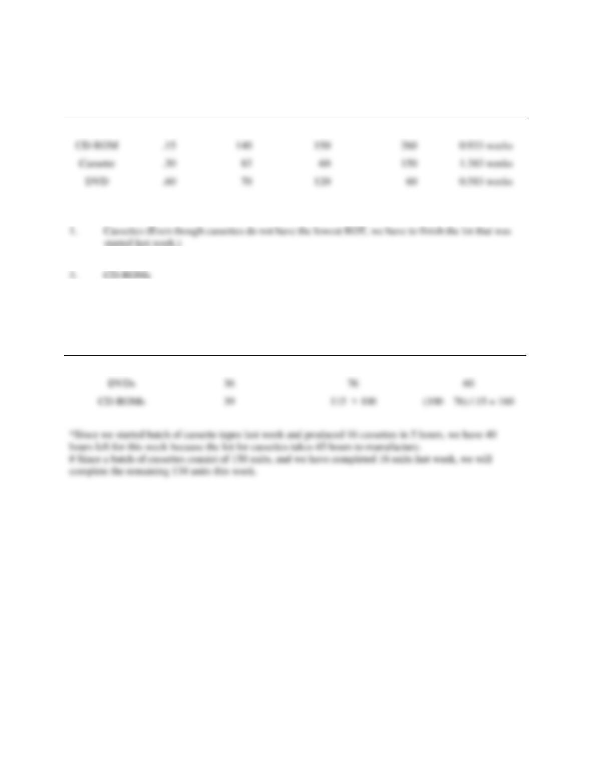
Based on the above calculations, the sequence of production in ascending order of runout times is:
1. CD-ROMs, 2. Diskettes, 3. DVDs, 4. Cassettes. Based on this order, the week’s production schedule
is summarized in the following table:
Sequence
Machine hours required
Cumulative
Machine hrs
Week’s production
schedule in units
CD–ROM
39
39
260 units
Diskettes
20
59
200 units
Note that we will exceed the weekly capacity after scheduling DVDs for production. The question is, how
many cassettes can we manufacture within the remaining time of the week? After producing DVDs, we
have 5 hours left (100 – 95) to manufacture the cassettes. Since each cassette takes .30 hours to
manufacture, the estimated number of cassettes we can manufacture during this week are 5 / .3 = 16.667
or 16 units.
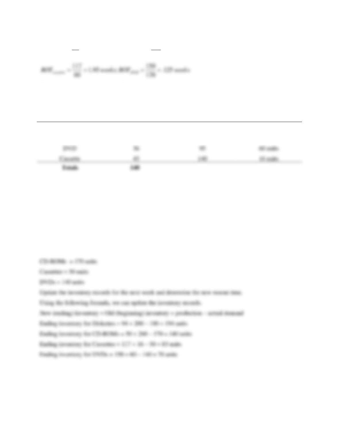
We would like to demonstrate the continuous nature of this process by showing the transition from one
week to another. Let’s assume that the time has passed, and the week has gone by. Kim checks the
company records and determines that the company has sold the following quantities of each item.
Diskettes = 100 units
Chapter 16 – Scheduling
16–38
Item
Production
time per unit
Inventory in
units
Forecasted
demand in units
Lot size in
units
Runout time in
weeks
Diskette
.10
194
85
200
2.28 weeks
Based on these updated runout times, the new sequence is as follows:
2. DVDs
4. Cassettes
5. Diskettes
Sequence
Machine hours required
Cumulative
Machine hours
Week’s production
schedule in units
Cassettes
40*
40
150 – 16 = 134#
Cassette
.30
83
60
150
1.383 weeks

Chapter 16 – Scheduling
16–39
Problems
1. Given the following data and 95 hours available per week for production, use the individual
runout time method of scheduling and determine the runout time sequence, batch production
times and scheduled production quantity for each product.
Product
Production time/unit
Lot size
Inventory on-hand
Forecasted demand
A
.25
160
120
100
2. Given the following data and 91 hours available per week for production, use the aggregate
runout time method of scheduling and determine the aggregate runout time, batch production
times and scheduled production quantity for each product.
Product
Production time/unit
Inventory on-hand
Forecasted demand
A
.25
120
100
B
.10
140
120
D
.30
100
C
.40
100
150
80
Chapter 16 – Scheduling
16–40
Solutions to problems
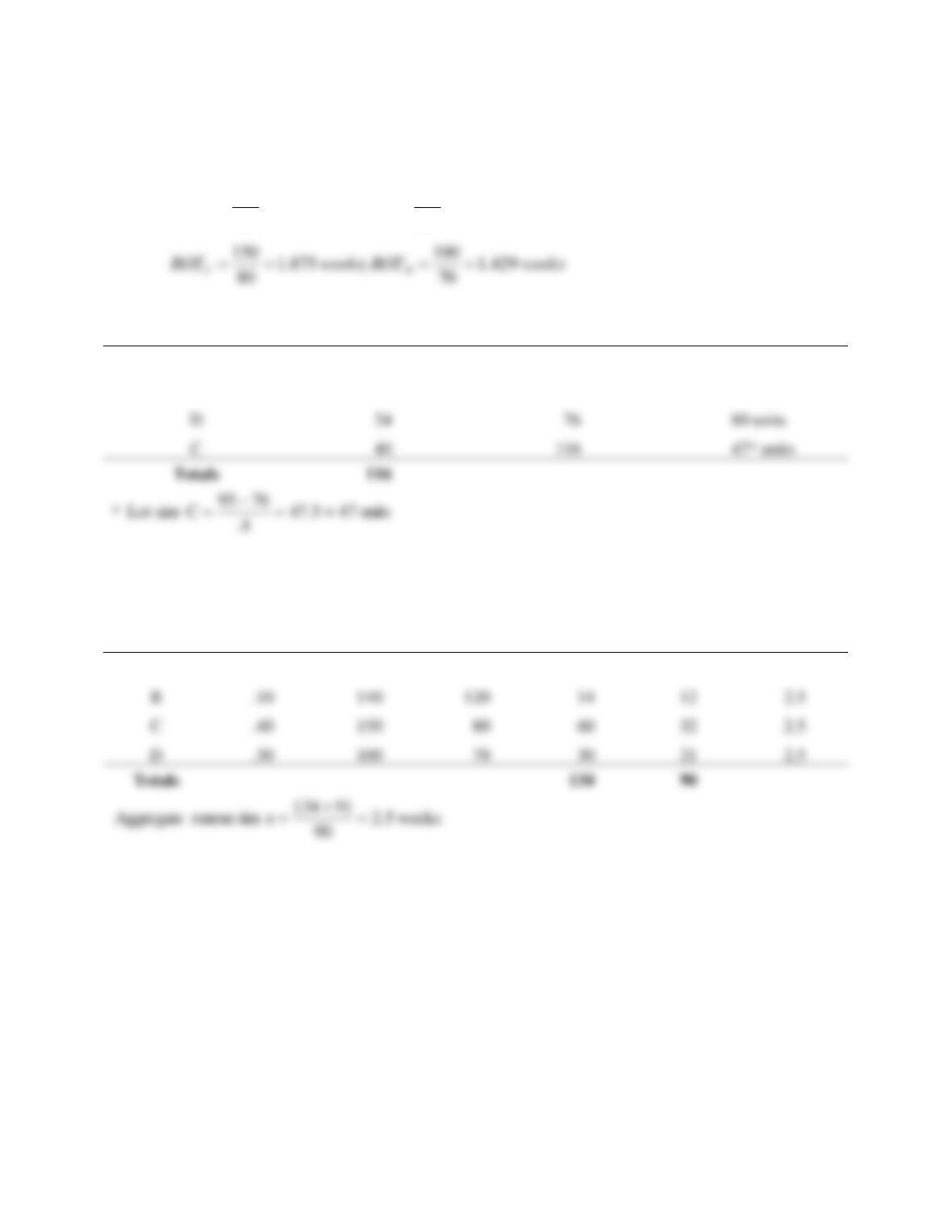
1.
weeks ROT weeks ROT
BA
16.1
120
140
;2.1
100
120
====
Sequence
Machine hours required
Cumulative
Machine hrs
Week’s production
schedule in units
B
12
12
120 units
A
40
52
160 units
D
24
76
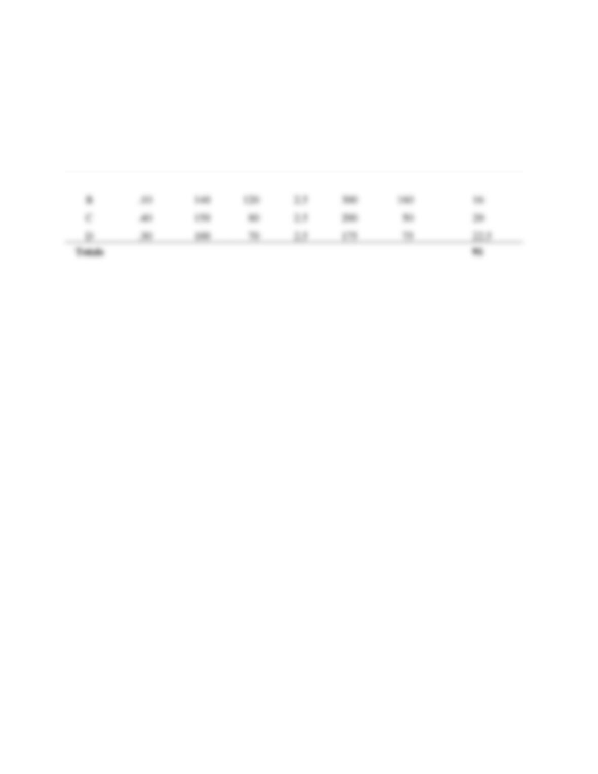
2.
Item
Production
time/unit
(hours)
Inventory
(units)
Forecasted
demand
(units)
Inventory
(hours)
Forecasted
demand
(hours)
Runout time
(in weeks)
A
.25
120
100
30
25
2.5
C
.40
150
60
32
2.5
Chapter 16 – Scheduling
16–41
Solutions to problems
2. continued
Item
Production
Time
(in hrs.)
(1)
Inventory
(in units)
(2)
Forecast
(in units)
(3)
ROT
(in
weeks)
(4)
# of
items
needed
(5) = (3)
x (4)
Production
schedule
(in units)
(6) =
(5) – (2)
Production
schedule
(in machine hrs).
(7) = (1) x (6)
A
.25
120
100
2.5
250
130
32.5