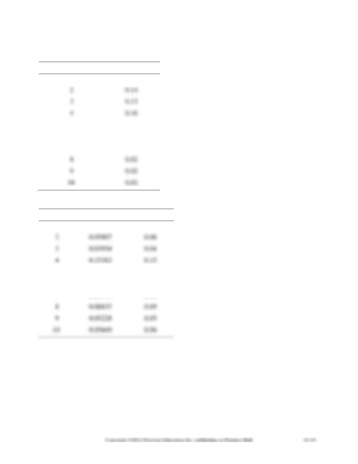
15-28. a. By using the Markov process, Sandy can determine market shares for each of the
quick-oil-change operations for next period. The results are summarized below.
State
Value
1
0.36
2
0.14
3
0.13
4
0.16
5
0.07
6
0.04
7
0.02
8
0.02
9
0.02
0.02
b. The equilibrium market shares for this problem are as follows:
State
Probability
Value
1
0.02439
0.02
2
0.05807
0.06
3
0.03934
0.04
4
0.15363
0.15
5
0.05226
0.05
6
0.41723
0.42
7
0.05779
0.06
8
0.08832
0.09
9
0.05228
0.05
0.05669
0.06
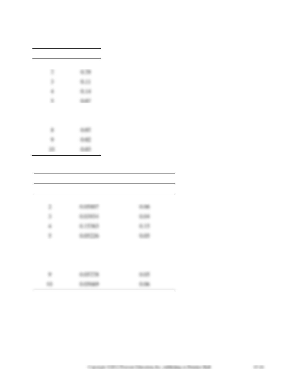
c. The market shares for next period will change, but the equilibrium shares will remain the
same. This is shown below:
State
Value
1
0.25
2
0.28
3
0.11
4
0.14
5
0.07
6
0.06
7
0.02
8
0.02
9
0.02
0.03
STEADY STATE
State
Probability
Value
1
0.02439
0.02
2
0.05807
0.06
3
0.03934
0.04
4
0.15363
0.15
5
0.05226
0.05
6
0.41723
0.42
7
0.05779
0.06
8
0.08832
0.09
9
0.05228
0.05
d. The equilibrium shares for this situation are given below. As you can see, shop 1 will not have 99% of the market in the long
run.
STEADY STATE
State
Probability
Value
1
0.50000
0.50
2
0.04762
0.05
3
0.01613
0.02
4
0.06494
0.06
5
0.02381
0.02
6
0.22112
0.22
7
0.02878
0.03
8
0.04333
0.04
9
0.02564
0.03
0.02864
0.03
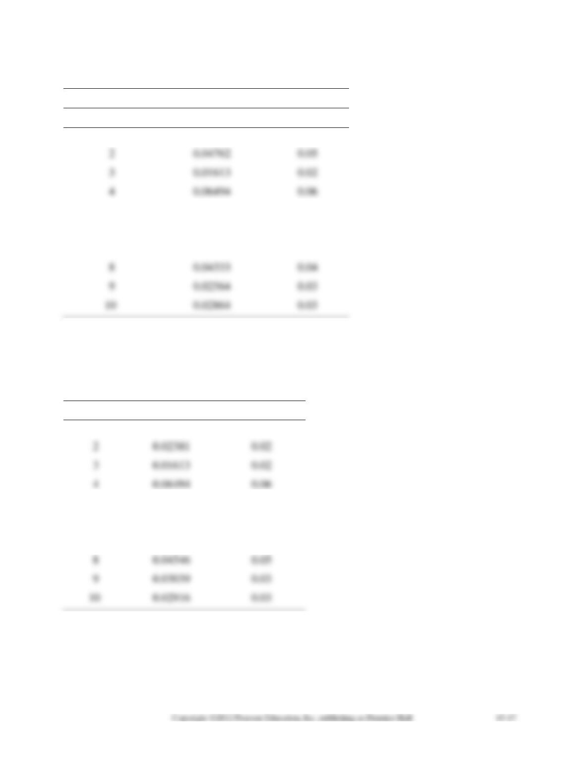
15-29. a. This is a typical Markov problem. We assume the same data as presented in Problem
15-28 with the exception that the first row for the matrix of transition (representing shop 1) will
have 0.99 in the first column and 0s elsewhere except for shop 7, which will have a 0.01. The
solution is given below. While Sandy has increased her market share, it is not 99%. She does not
win her bet.
States
Probability
Value
1
0.50000
0.50
2
0.02381
0.02
3
0.01613
0.02
4
0.06494
0.06
5
0.02381
0.02
6
0.22112
0.22
7
0.04519
0.05
8
0.04546
0.05
9
0.03039
0.03
0.02916
0.03
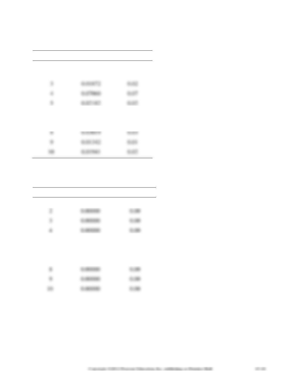
b. We make the same types of changes for Chris that we did for Sandy. The seventh row for the matrix of transition (representing
shop 7) will have 0.99 in the seventh column and zeros elsewhere except for shop 1, which will have a 0.01. The solution is given
below. As with part (a), Chris has also increased his market share, but it is not 99%. He does not win his bet.
States
Probability
Value
1
0.02439
0.02
2
0.02763
0.03
3
0.01872
0.02
4
0.07060
0.07
5
0.02182
0.02
6
0.13449
0.13
7
0.63934
0.64
8
0.03019
0.03
9
0.01342
0.01
10
0.01941
0.02
c. If both are correct, the market shares will be 50% each as seen in the following solution.
Perhaps they can get together, each paying for his or her own meal. Neither Sandy or Chris
will end up with 99% of the market.
States
Probability
Value
1
0.50000
0.50
2
0.00000
0.00
3
0.00000
0.00
4
0.00000
0.00
5
0.00000
0.00
6
0.00000
0.00
7
0.50000
0.50
8
0.00000
0.00
9
0.00000
0.00
10
0.00000
0.00
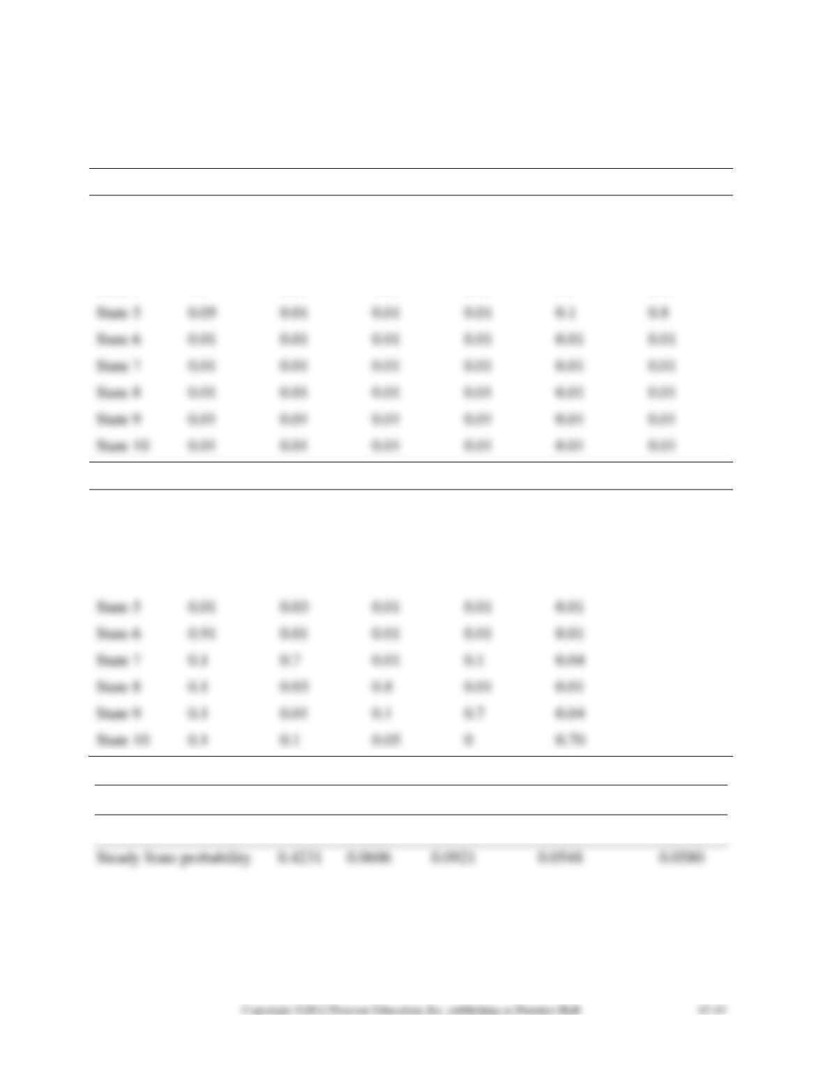
15-30. Changing the first row will have an impact on the steady-state market shares. To see the
impact, we can use QM for Windows to solve this problem. The results are presented below.
Data
Initial
State 1
State 2
State 3
State 4
State 5
State 1
0.6
0.73
0.03
0.03
0.03
0.03
State 2
0.1
0.01
0.8
0.01
0.01
0.01
State 3
0.1
0.01
0.01
0.7
0.01
0.01
State 4
0.1
0.01
0.01
0.01
0.9
0.01
State 5
0.05
0.01
0.01
0.01
0.1
0.8
State 6
0.01
0.01
0.01
0.01
0.01
0.01
State 7
0.01
0.01
0.01
0.01
0.01
0.01
State 8
0.01
0.01
0.01
0.01
0.01
0.01
State 9
0.01
0.01
0.01
0.01
0.01
0.01
State 10
0.01
0.01
0.01
0.01
0.01
0.01
State 6
State 7
State 8
State 9
State 10
State 1
0.03
0.03
0.03
0.03
0.03
State 2
0.1
0.01
0.01
0.01
0.03
State 3
0.1
0.01
0.05
0.05
0.05
State 4
0.01
0.01
0.01
0.01
0.02
State 5
0.01
0.03
0.01
0.01
0.01
State 6
0.91
0.01
0.01
0.01
0.01
State 7
0.1
0.7
0.01
0.1
0.04
State 8
0.1
0.03
0.8
0.01
0.01
State 9
0.1
0.01
0.1
0.7
0.04
State 10
0.1
0.1
0.05
0
0.70
Results State 1 State 2 State 3 State 4 State 5
Steady State probability 0.0357 0.0510 0.0346 0.1391 0.0510
State 6 State 7 State 8 State 9 State 10
SOLUTIONS TO INTERNET HOMEWORK PROBLEMS
15-31. Let states 1, 2, 3 represent fair, tolerable, and miserable traffic conditions, respectively:
0.7 0.2 0.1
0.2 0.75 0.05
0.3 0.1 0.6
P
=
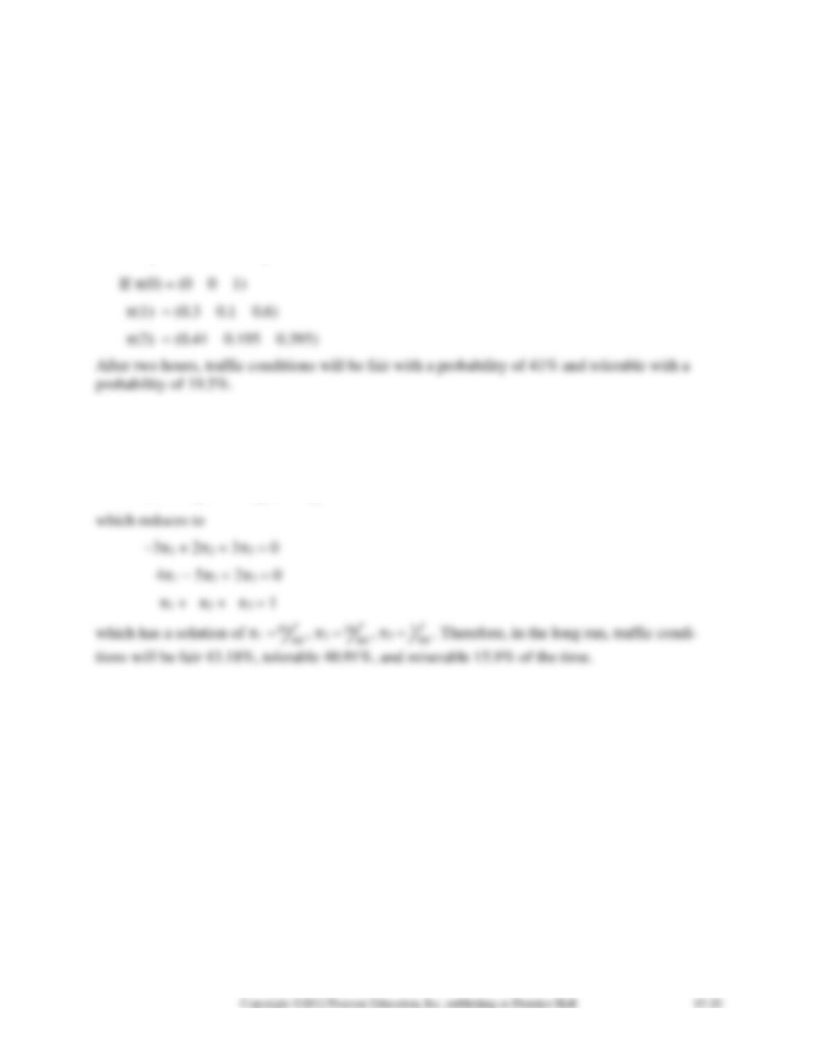
15-32. From Problem 15-31 we get the transition matrix P. In the long run, = P:
1 = 0.71 + 0.22 + 0.33
2 = 0.21 + 0.752 + 0.13
1 = 1 + 2 + 3
15-33. Let existence in Lake Jackson denote state 1 and existence in Lake Bradford denote state
2 for an individual tiger minnow. Then:
0.9 0.1
0.05 0.95
P
=
Also:
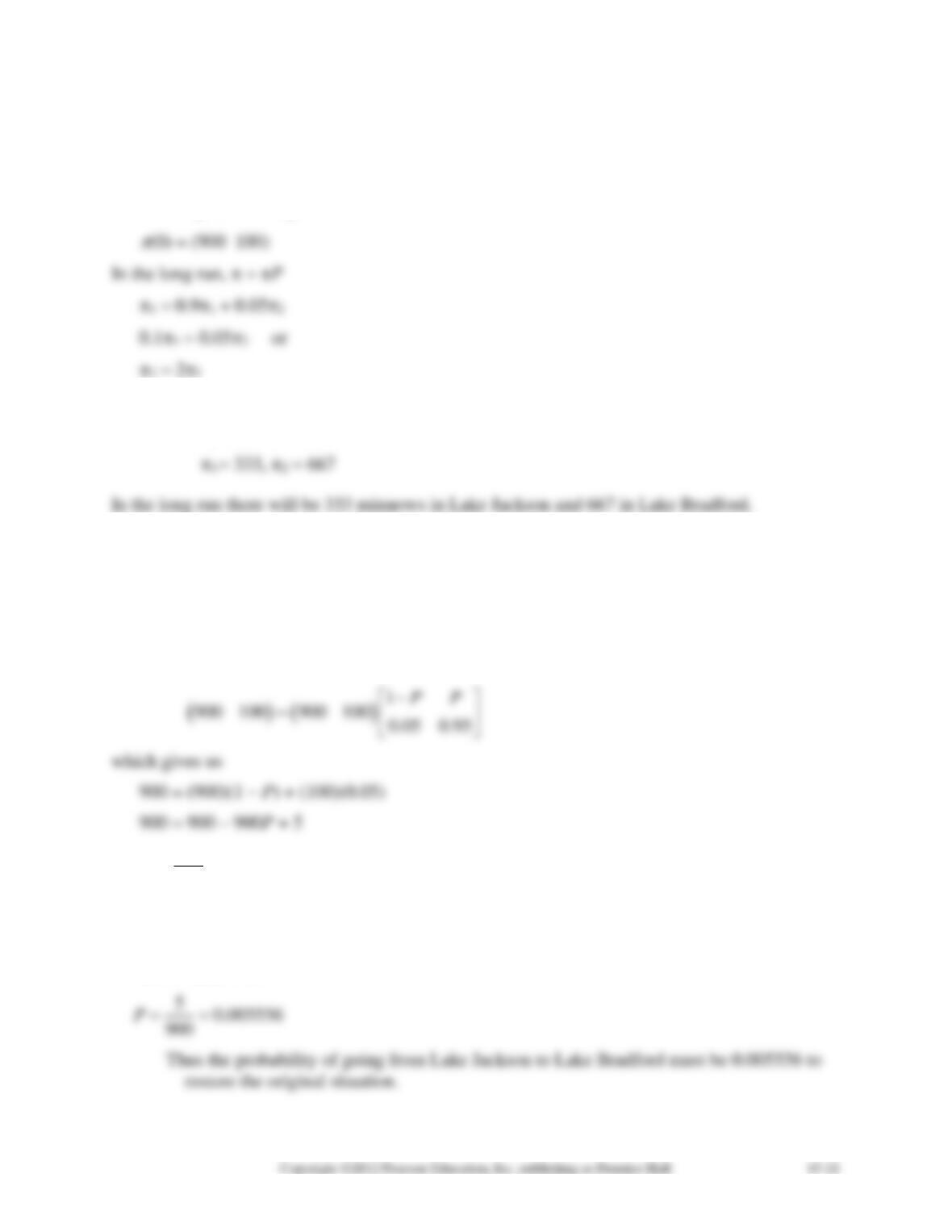
1 + 2 = 1,000
15-34. Original state = (900 100) = (0)
Let P = probability of going from Lake Jackson to Lake Bradford.
1
0.05 0.95
PP
P−
=
At equilibrium, = P
50.005556
900
P==
Here is another way of solving the problem:
100 = (900)(P) + (100)(0.95)
100 = 900P + 95
50.005556
900
P==
SOLUTIONS TO RENTALL TRUCKS CASE
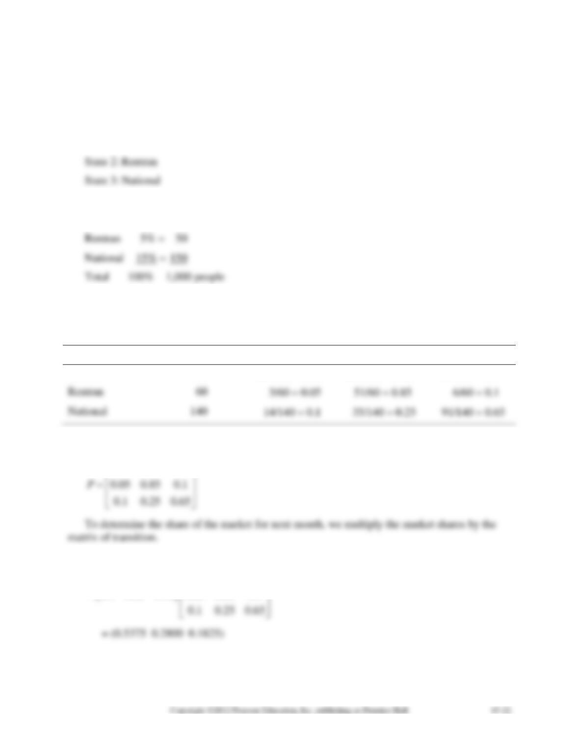
1. To determine what the market shares will be in one month, Markov analysis must be used.
We will define the following states for this case:
State 1: Rentall
The market shares are as follows:
Rentall 80% = 800
Therefore,
n(0) = (0.8 0.05 0.15)
The next step is to determine the matrix of transition. If no changes are made, one has:
Customers
Rentall
Rentran
National
Rentall
800
520/800 = 0.65
200/800 = 0.25
80/800 = 0.1
National
140
91/140 = 0.65
Thus
0.65 0.25 0.1
n(1) = n(0)P
( )
0.65 0.25 0.1
0.8 0.05 0.15 0.05 0.85 0.1
=
Thus the new share of the market is about
Rentall 54%
If changes are made:
Customers
Rentall
Rentran
National
Rentall
800
680/800 = 0.85
100/800 = 0.125
20/800 = 0.025
Rentran
60
9/60 = 0.15
45/60 = 0.75
6/60 = 0.10
National
140
28/140 = 0.2
35/140 = 0.25
77/140 = 0.55
0.85 0.125 0.025
n(1) = n(0)P
0.85 0.125 0.025
Market shares:
Rentall 72%
Rentran 17%
National 11%
Total 100%
2. With no changes, in two months the market shares will be
In three months, the market share will be
The approximate market shares after three months are listed below.
Rentall 29%
Rentran 50%
National 21%
Total 100%
If the changes are made,
n(2) = n(1)P
0.85 0.125 0.025
n(3) = n(2)P
0.85 0.125 0.025
3. At equilibrium, with these changes,
( ) ( )
1 2 3 1 2 3
0.85 0.125 0.025
0.15 0.75 0.10
0.2 0.25 0.55
n n n n n n
=
n1 = 0.85n1 + 0.15n2 + 0.2n3
n2 = 0.125n1 + 0.75n2 + 0.25n3
We have four equations and three unknowns. We drop equation 1 and solve equations 2, 3, and 4
for n1, n2, and n3.
The results are
n1 = 0.519
The equilibrium market shares are
Rentall 52%
With no changes,
( ) ( )
1 2 3 1 2 3
0.65 0.25 0.1
0.05 0.85 0.1
0.2 0.25 0.65
n n n n n n
=
Solving as above, the results are
n1 = 0.153
The equilibrium market shares would be
Rentall 15%
SOLUTIONS TO INTERNET CASES
University of Texas–Austin
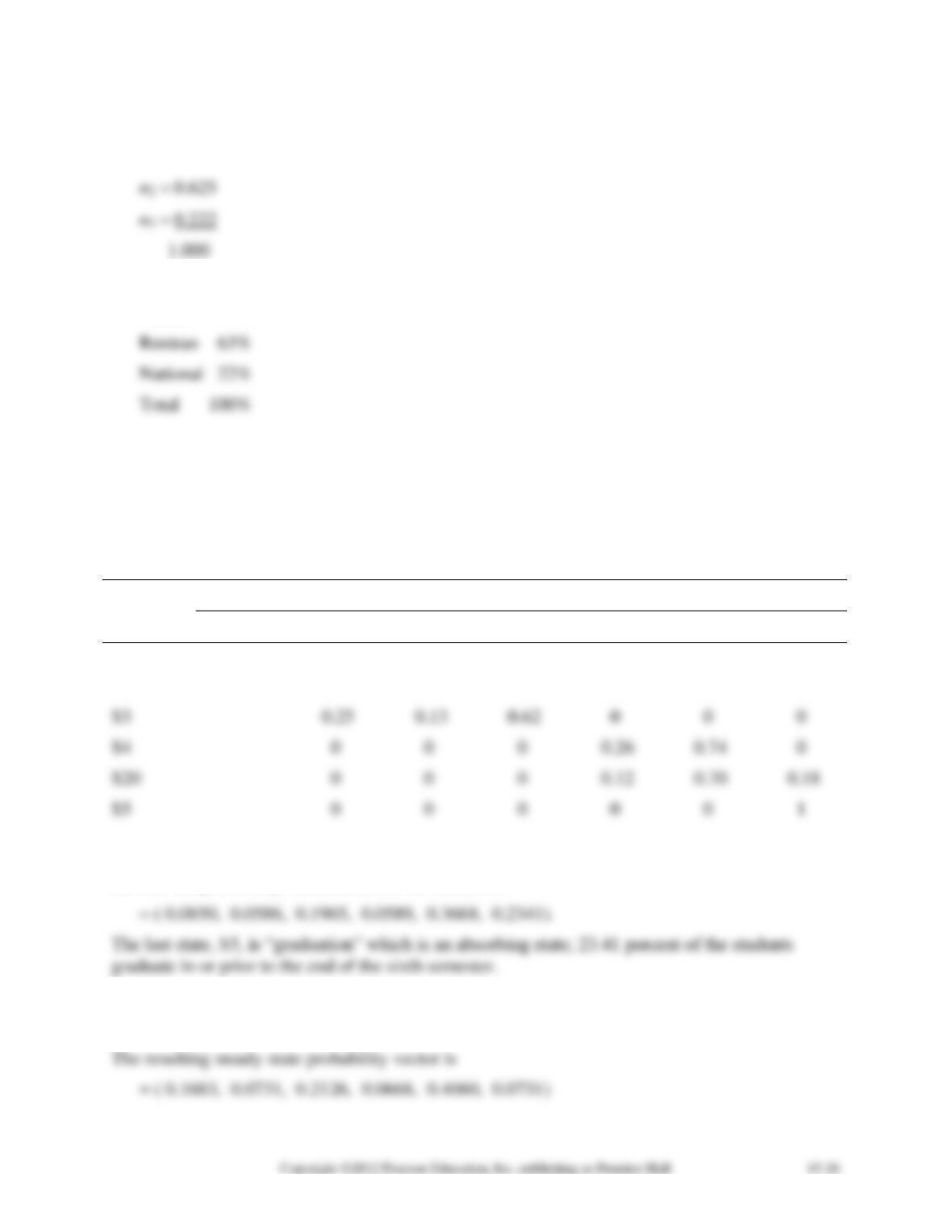
1. The transition probabilities of Figure 1 lead to the following Markov transition matrix, M:
To
S1
S2F
S3
S4
S20
S5
From
S1
0.25
0.27
0.48
0
0
0
S2F
0
0
0
0.01
0.99
0
S3
0.25
0.13
0.62
0
0
0
S4
0
0
0
0.26
0.74
0
S20
0
0
0
0.12
0.70
0.18
S5
0
0
0
0
0
1
A student beginning the program corresponds to the vector v = (1, 0, 0, 0, 0, 0). After six se-
mesters the probability distribution for the student is:
2. The balance assumption replaces the last row of the M matrix with
S5 1 0 0 0 0 0.
3. The Markov assumption states that the chance of going from one state to another depends on-
ly upon the state one is in and not on how the individual reached that state. Thus, a student who
has withdrawn after advancement (state S4) and has remained in that state for a number of se-
mesters is just as likely to re-enroll in the program as a student who has just withdrawn, if the
Markov assumption is true. In practice, one would have to obtain data to support this assumption.
St. Pierre Salt Company
The case illustrates the use of Markov analysis. Assumptions for a Markov process are:
a) The probability of going to each state depends only on the current state and not on the
manner in which the current state was reached.
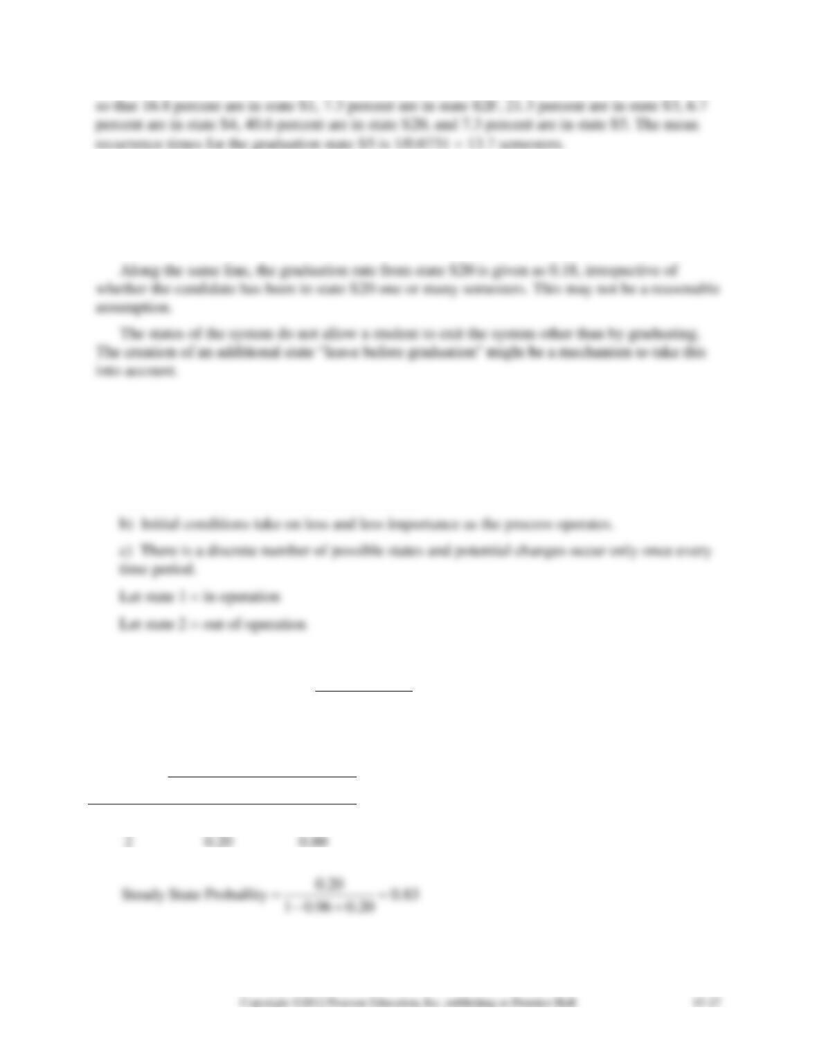
From Markov analysis we define the “steady state” probability as:
( ) ( )
( ) ( )
2
1 on day given 1 on day 1 1 1 2
p
pm pp
=−+
For the AKZ centrifuge:
To
From
1
2
1
0.96
0.04
2
0.20
0.80
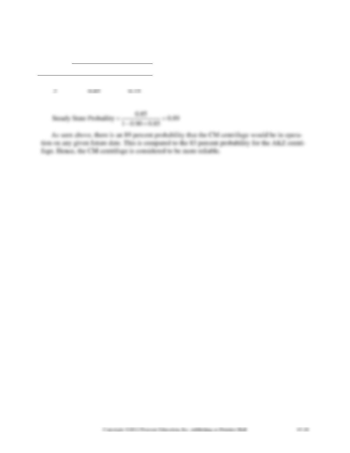
For the CM centrifuge:
To
From
1
2
1
0.90
0.10
2
0.85
0.15