15-32 CHAPTER 15: MARKOV CHAINS
A B C
19. P =
10 0
010
.3 .1 .6
A
B
C
, P4 ≈
100
010
.6528 .2176 .1296
, P8 ≈
10 0
01 0
.7374 .2458 .01680
,
.7498 .2499 0
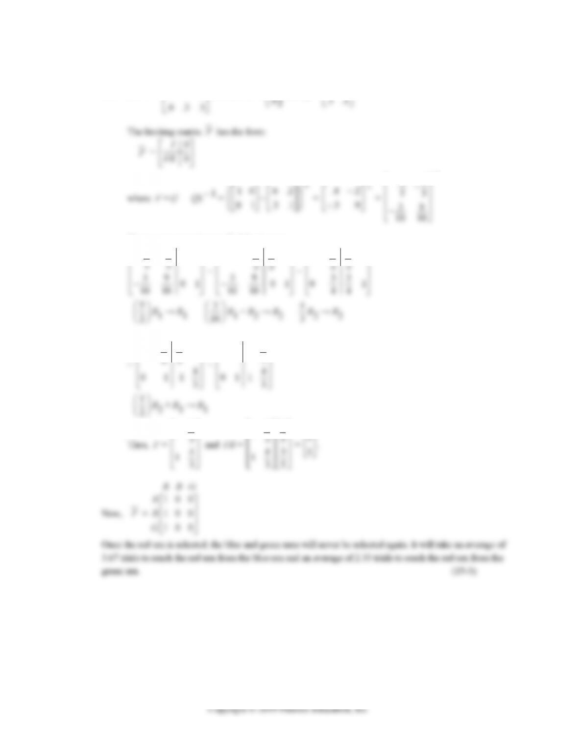
.75 .25 0
C
A B C D
20. P =
1000
0100
.1 .5 .2 .2
.1 .1 .4 .4
A
B
C
D
, P4 ≈
1000
0100
.1784 .7352 .0432 .0432
.2568 .5704 .0864 .0864
,
8 ≈
1000
0100
1000
0100
.2 .8 0 0
.3 .7 0 0
C
D
21. A standard form for the given matrix is:
B D A C
1000
B
22. We will determine the limiting matrix of:
A B C
P =
010
001
A
B
.2 .6 .2
CHAPTER 15 REVIEW 15-33
The corresponding system of equations is:
.2s3 = s1 s1 – .2s3 = 0
s
1 + .6s3 = s2 or s1 – s2 + .6s3 = 0
s2 + .2s3 = s3 s2 – .8s3 = 0
.1 .4 .5
C
(A) [0 0 1]
.1 .4 .5
.1 .4 .5
= [.1 .4 .5]
A
BC
A
.1 .4 .5
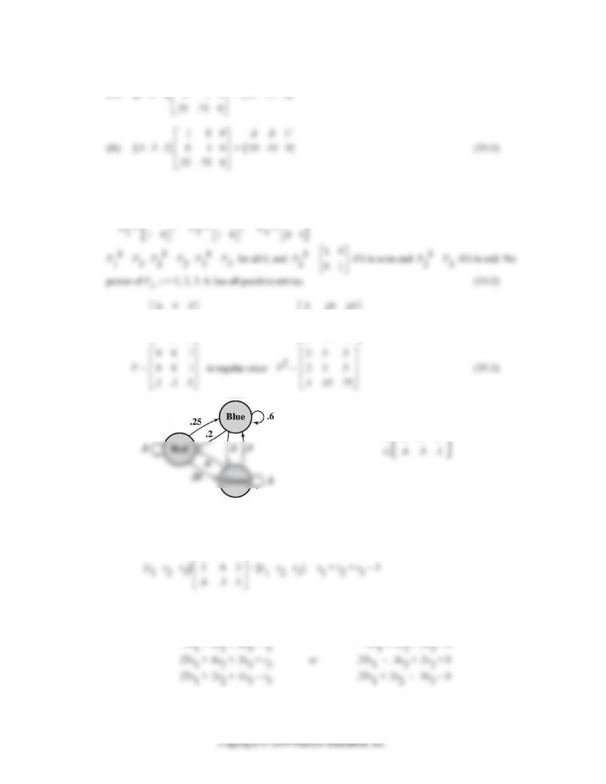
23. The transition matrix:
A B C
P =
100
010
A
B
.25 .75 0
C
15-34 CHAPTER 15: MARKOV CHAINS
(A) [0 0 1]
100
010
= [.25 .75 0]
A
BC
A
.25 .75 0
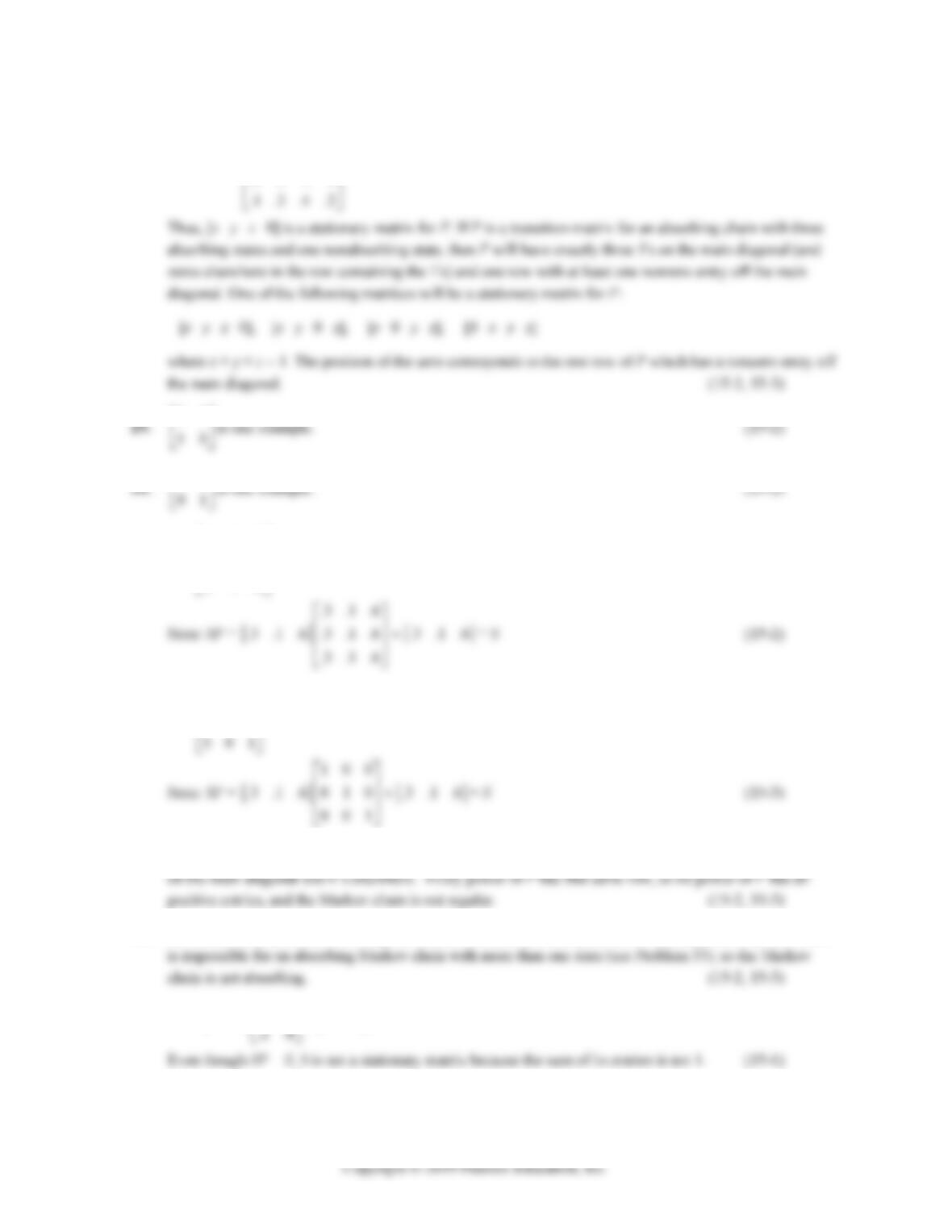
24. No. If P is a transition matrix with 2 entries equal to 0, then P has one of the forms: P1 = 10
01
,
25. Yes; P =
.5 0 .5
.5 .5 0
is regular since P2 =
.25 .5 .25
.25 .25 .5
001
.2 .3 .5
.2 .3 .5
.1 .15 .75
26. (A)
(B) P = .5 .25 .25
.2 .6 .2
RBG
R
B
(C) The chain is regular since it has only positive entries.
(D) Let
S = [s1 s2 s3] and solve the system:
.5 .25 .25
which is equivalent to:
s1 + s2 + s3 = 1 s1 + s2 + s3 = 1
CHAPTER 15 REVIEW 15-35
We use row operations to solve this system; but first multiply the
second, third and fourth equations by 10 to simplify the
calculations.
1111
5260
11 11
07115
1111
01235
5
2
R1 + R3 → R3 R2 ↔ R4
13
2
R2 + R3 → R3
00 150 30
000 0
1
150 R3 → R3 22R3 + R1 → R1
The solution is s1 = 0.4, s2 = 0.4, s3 = 0.2 and
R B G
.4 .4 .2
R
green urn 20% of the time. (15-2)
27. (A)
RBG
R
(C) State R is an absorbing state. The chain is absorbing since it is possible to go from states B and
15-36 CHAPTER 15: MARKOV CHAINS
(D) For P =
100
.2 .6 .2
we have R = .2
and Q = .6 .2
.
We use row operations to find the inverse:
21
10
15
10
15
10
15
10
22
2
103 3
CHAPTER 15 REVIEW 15-37
28. [x y z 0]
1000
0100
0010
= [x y z 0]
31. P =
.3 .1 .6
.3 .1 .6
.3 .1 .6
is one example.
.3 .1 .6
.3 .1 .6
32. P =
100
010
is one example.
100
001
33. If P is the transition matrix of an absorbing Markov chain with more than one state, then P has a row with 1
34. If P is the transition matrix of a regular Markov chain, then some power of P has all positive entries. This
35. SP =
.4 .6
.3 .9 .3 .9 ;
15-38 CHAPTER 15: MARKOV CHAINS
A B C D
.2 .3 .1 .4
0010
A
B
For example
0.2.75.05
0.8 0 .2
0.6.25.15
00 1 0
A B C D A B C D
.1 0 .3 .6
.2 .4 .1 .3
A
B
.392 .163 .134 .311
.392 .163 .134 .311
A
B
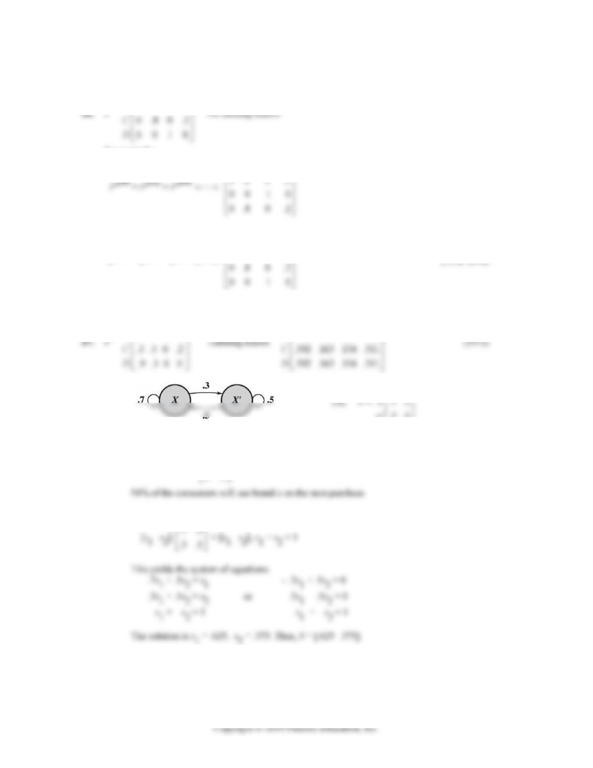
38. (A)
‘
‘.5.5
x
x
x
(C)
S = [.2 .8]
(D) S1 = SP = [.2 .8] .7 .3
= [.54 .46]
(E) To find the stationary matrix S = [s1 s2], we need to solve:
(F) Brand X will have 62.5% of the market in the long run. (15-2)
CHAPTER 15 REVIEW 15-41
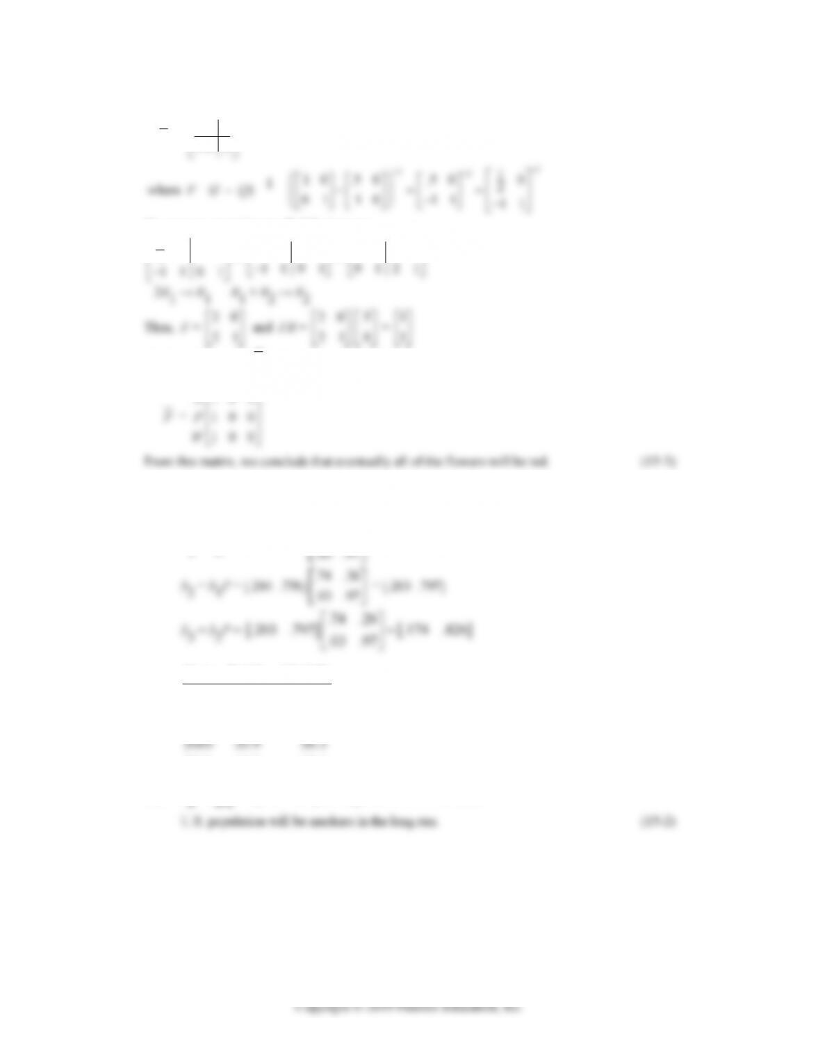
The limiting matrix for P will have the form:
P = 0
0
I
FR
1
111
10 .50 .50 0
01 10 11 11
We use row operations to find the inverse:
1010
2
~ 1020
~ 1020
The limiting matrix P is:
R P W
100
R
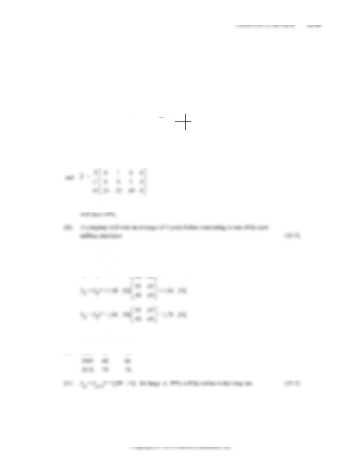
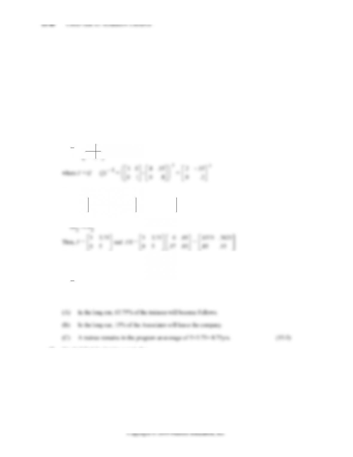
43. (A) P = .74 .26
.03 .97
, S0 = [.301 .699]
S1 = S0P = [.301 .699] .74 .26
= [.244 .756]
(B)
Year Data% Model%
1985 30.1 30.1
1995 24.7 24.4
2010 19.3 17.4
(C) Sn = Sn-1P ≈ [.103 .897] for large n; 10.3% of the adult