15-1
15 MARKOV CHAINS
EXERCISE 15-1
69
6945
6. 469
not defined. 8. 694 2445 69
.7 .3 .7 .3
.7 .3 .7 .3
.7 .3 .7 .3
The transition matrix for Problems 15–20 is
A B
.5 .5
.8 .2
A
B
.5 .5 .5 .5
18.
12
.5 .5 .5 .5
.9 .1 .53 .47 , .53 .47 .641 .359
SS
20.
12
.5 .5 .5 .5
.2 .8 .74 .26 , .74 .26 .578 .422
SS
22.
12
.2 .4 .4 .2 .4 .4
0 0 1 .7 .2 .1 .5 .3 .2 , .5 .3 .2 .7 .2 .1 .41 .32 .27
SS
24.
12
.2 .4 .4 .2 .4 .4
.5 .5 0 .7 .2 .1 .45 .3 .25 , .45 .3 .25 .7 .2 .1 .425 .315 .26
SS
.2 .4 .4 .2 .4 .4
15-2 CHAPTER 15: MARKOV CHAINS
The transition matrix for problems 27–32 is
.2 .3 .5
.4 .2 .4
.2 .3 .5 .2 .3 .5
30.
12
.2 .3 .5 .2 .3 .5
.8 0 .2 .1 .8 .1 .24 .28 .48 , .24 .28 .48 .1 .8 .1 .268 .392 .34
SS
.2 .3 .5 .2 .3 .5
34. The transition matrix for Problems 15–20 is
A B
.8 .2
A
36.
38. .9 .1
.4 .8
40. 01
10
42.
.2 .8
.5 .5
EXERCISE 15-1 15-3
44.
.3 .3 .4
.7 .2 .2
46.
A B
.8 .2
B
48. No. Choose any x, 0 ≤ x ≤ 1, then any
A B
.3 .7
B
50.
.1 .8 .1
C
52. a + 0 + .9 = 1 implies a = .1
54. 0 + 1 + a = 1 implies a = 0
56. No. a + .8 + .1 = 1 implies a = .1
15-4 CHAPTER 15: MARKOV CHAINS
58.
A B
.6 .4
A
60.
10 0
C
62. Using P2, the probability of going from state B to state C in two trials is the (2,3) position: .38.
64. Using P3 the probability of going from state B to state B in three trials is the (2,2) position: .336.
66. S2 = S0P2 = [0 1 0]
.43 .35 .22
.25 .37 .38
= [.25.37.38]
ABC
68. S3 = S0P3 = [1 0 0]
.35 .348 .302
.262 .336 .402
= [.35.348.302]
A
BC
70. n = 11
72. P = .8 .2
.3 .7
, P2 = .8 .2
.3 .7
.8 .2
.3 .7
= .7 .3
.45 .55
.5625 .4375
EXERCISE 15-1 15-5
74. P =
010
.8 0 .2
10 0
, P2 =
010
.8 0 .2
10 0
010
.8 0 .2
10 0
=
.8 0 .2
.2 .8 0
010
,
.2 .8 0
76. Sk = S0Pk = [0 1]Pk; the entries in Sk are the entries in the second row of Pk.
78. (A) P2 =
.5 .3 .1 .1
0100
0010
.5 .3 .1 .1
0100
0010
.26.47.18.09
0100
.09 .31 .43 .17
P4 = P2·P2 =
.26 .47 .18 .09
0100
0010
.26.47.18.09
0100
0010
00 10
.0387 .405 .5193 .037
C
D
(B) The probability of going from state A to state D in 4 trials
(C) The element in the (3,2) position: 0
(D) The element in the (2,1) position: 0
80. If P = 1
1
aa
bb
is a probability matrix,
then 0 ≤ a ≤ 1, 0 ≤ b ≤ 1.
aa
15-6 CHAPTER 15: MARKOV CHAINS
Copyright © 2019 Pearson Education, Inc.
Now,
ac + (1 – b)(1 – c) ≥ 0, c(1 – a) + b(1 – c) ≥ 0 since 0 ≤ c ≤ 1 also. Furthermore,
ac + (1 – b)(1 – c) + c(1 – a) + b(1 – c)
= ac + 1 – c – b + bc + c – ac + b – bc = 1.
Thus, SP is a probability matrix.
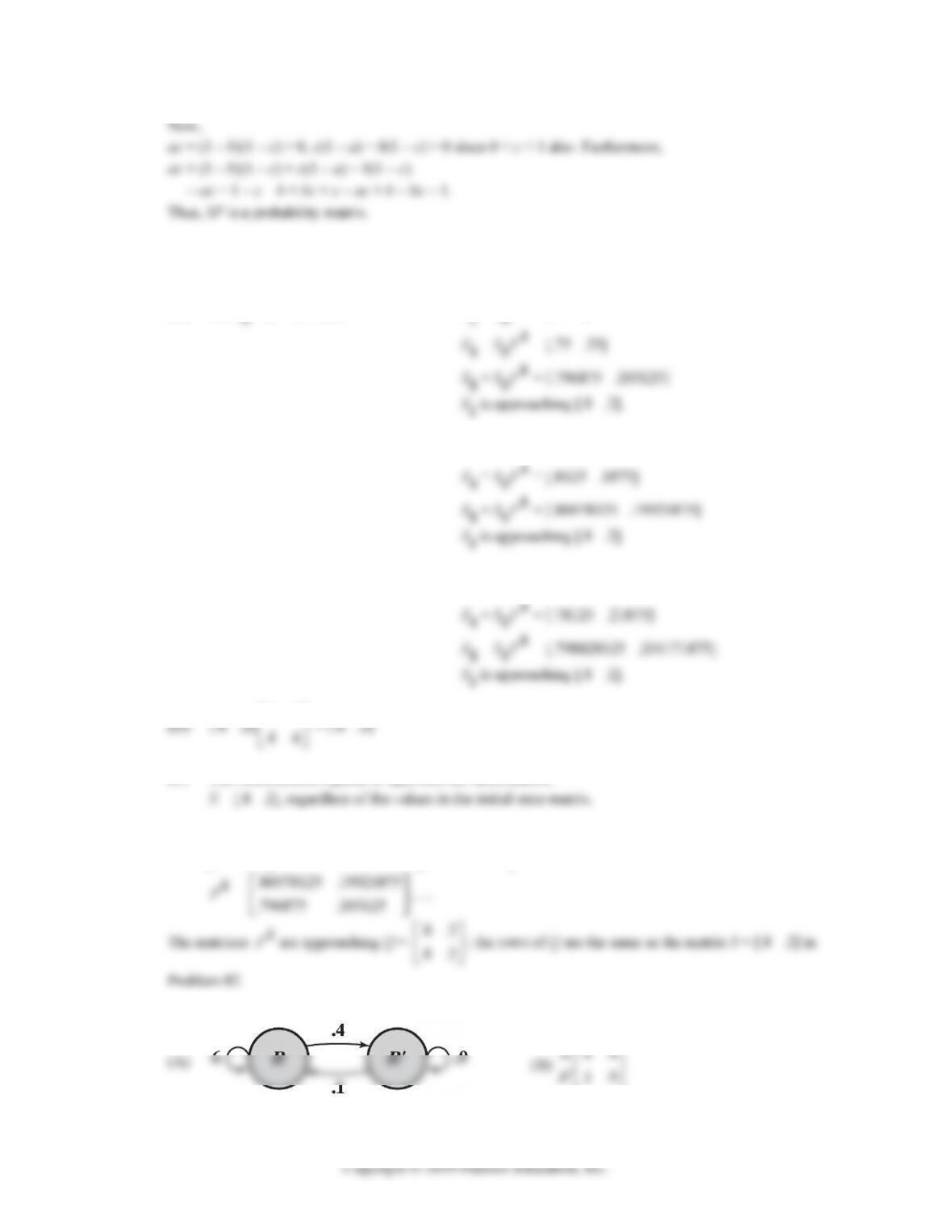
82. P = .9 .1
.4 .6
(A) Let S0 = [0 1]. Then S2 = S0P2 = [.6 .4]
(B) Let S0 = [1 0]. Then S2 = S0P2 = [.85 .15]
(C) Let S0 = [.5 .5]. Then S2 = S0P2 = [.725 .275]
(E) The state matrices appear to approach the same matrix,
84. P2 = .85 .15
.6 .4
, P4 = .8125 .1875
.75 .25
,
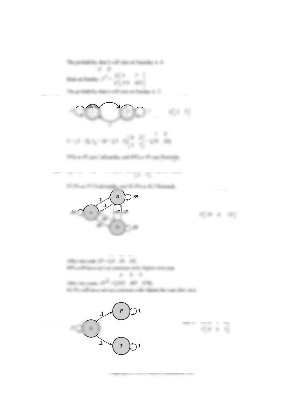
86. Let R = denote “rain” and R‘ “not rain”.
R R’
.1 .9
R
R
EXERCISE 15-1 15-7
R R‘
(C) Rain on Saturday: P2 = .4 .6
.15 .85
R
R
88. (A)
.2
L K
.8 .2
L
90. (A)
A B N
(B) P =
.85 .1 .05
.1 .85 .05
A
B
A B N
(C) S = [.25 .3 .45]
(D) From part (C), we get 46% and 48.7% respectively.
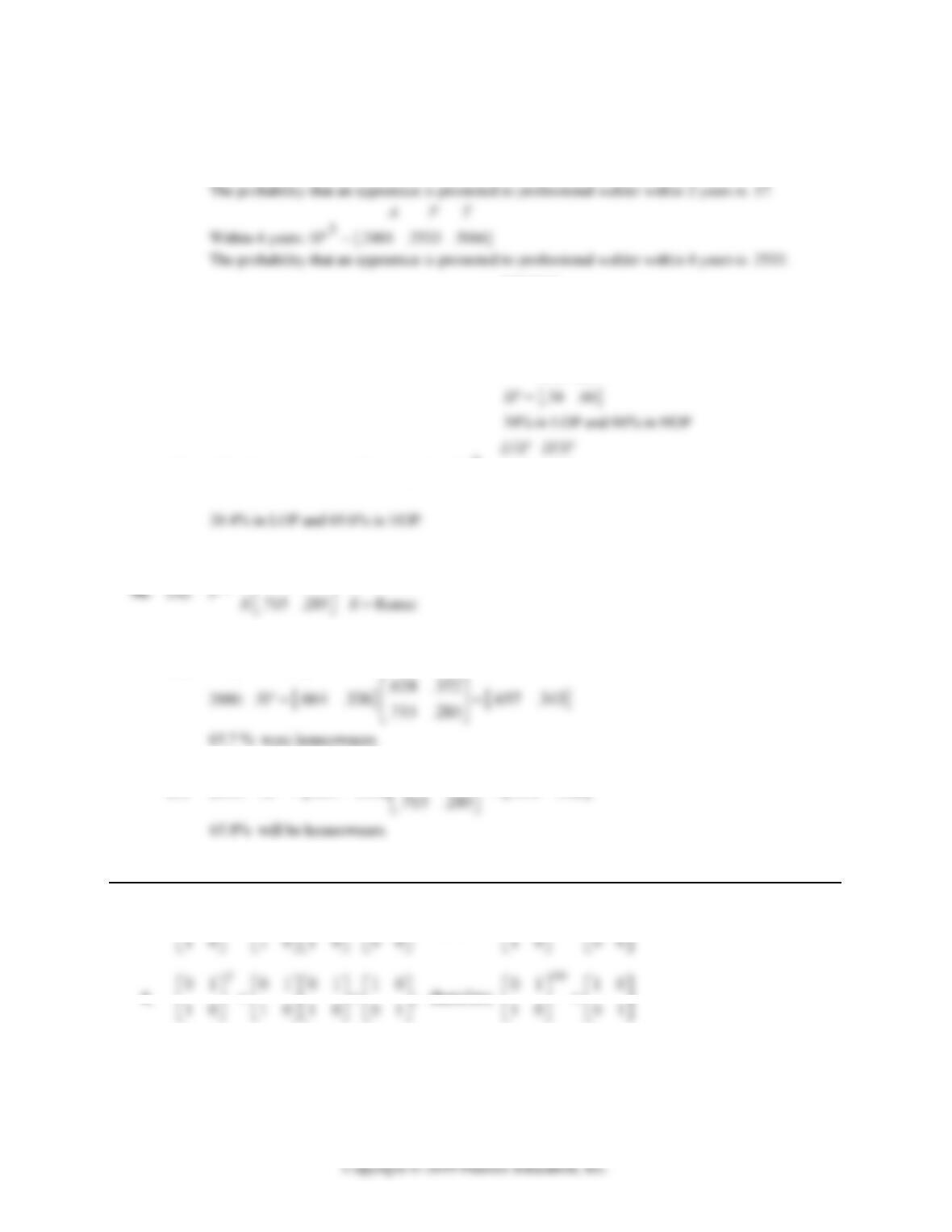
92. (A)
A P T
.7 .1 .2
A
15-8 CHAPTER 15: MARKOV CHAINS
(C) S = [.7 .1 .2]
A P T
within 2 years: SP = [.49 .17 .34]
LOP HOP
94. (A) P = LOP .7 .3
HOP .1 .9
(B) S =
.4 .6
L
OP HOP
After last open enrollment period:
LOP HOP
(C) After the next open enrollment period: SP2 = [.304 .696]
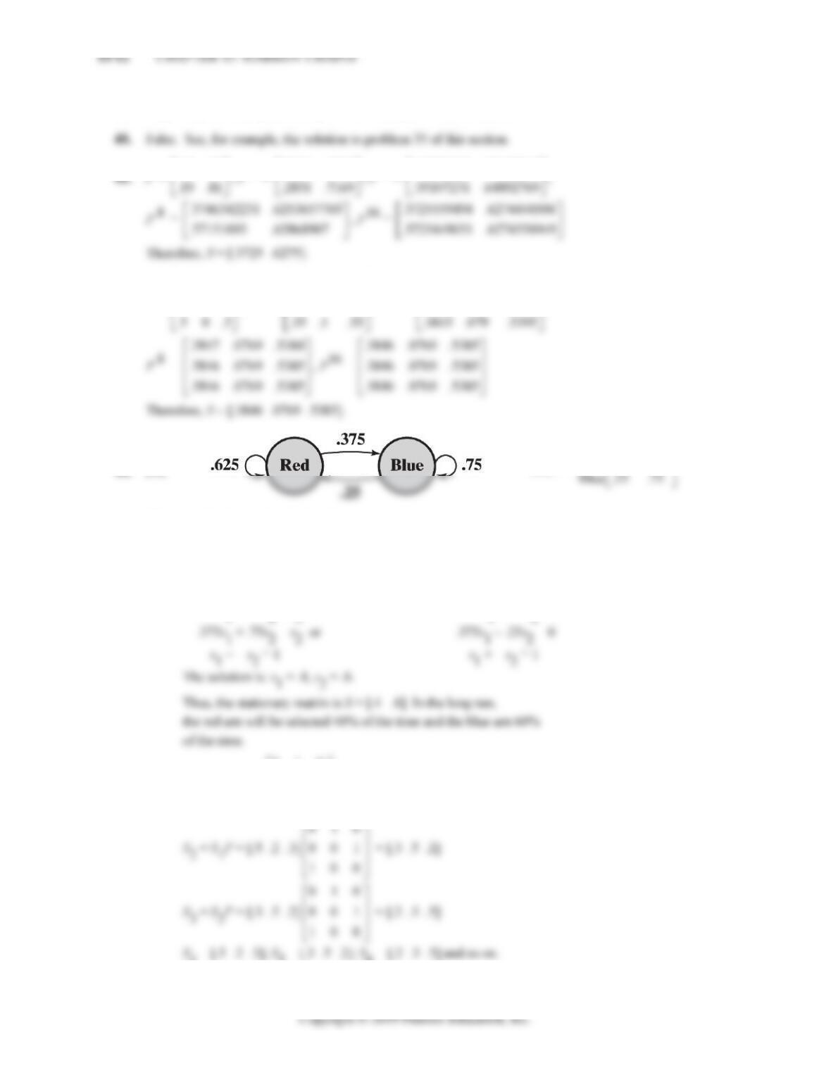
H R
HH
H R
(B) S = [.664 .336]
.628 .372
(C) 2030:
3
3.628 .372
.664 .336 .658 .342
SP
EXERCISE 15-2
2.
2100
00 0000 00 00 00
; therefore
4.
; therefore
EXERCISE 15-2 15-9
6.
100
100100 100 100 100
010010 010;Therefore 010 010
8.
001001 000; 001=001000=000;
10. .3 .7
12. P = .5 .5
14. P = .4 .6
10
.4 .6
16. .3 .7
18. .2 .5 .3
20. P =
00 1
.7 0 .3
15-10 CHAPTER 15: MARKOV CHAINS
22. P =
00 1
.9 0 .1
.09 .9 .01
24. Let S = [s1 s2], and solve the system:
[s1 s2].8 .2
.3 .7
= [s1 s2], s1 + s2 = 1
which is equivalent to
.8s1 + .3s2 = s1 –.2s1 + .3s2 = 0
.6 .4
26. Let S = [s1 s2], and solve the system:
[s1 s2].9 .1
.7 .3
= [s1 s2], s1 + s2 = 1
which is equivalent to
.875 .125
28. Let S = [s1 s2 s3], and solve the system:
.4 .1 .5
EXERCISE 15-2 15-11
From the first and third equations, we have s2 = 3s1, and s3 = s1.
Substituting these values into the fourth equation, we get:
.2 .6 .2
30. Let S = [s1 s2 s3], and solve the system:
[s1 s2 s3]
.2 .8 0
.6 .1 .3
0.9.1
= [s1 s2 s3], s1 + s2 + s3 = 1
which is equivalent to
.2
s1 + .6s2 = s1 –.8s1 + .6s2 = 0
From the first and third equations, we have s1 = 3
4s2, and s3 = 1
3s2.
Substituting these values into the fourth equation, we get:
36. True, such a matrix would satisfy all of the conditions of the definition.
EXERCISE 15-2 15-13
Copyright © 2019 Pearson Education, Inc.
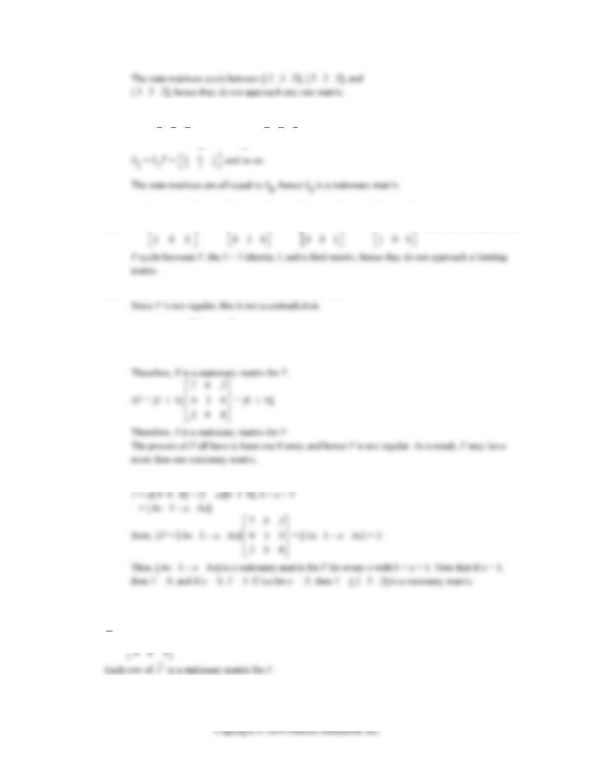
The state matrices cycle between [.2 .3 .5], [.5 .2 .3], and
[.3 .5 .2], hence they do not approach any one matrix.
(B) S1 = 111
333
010
001
100
= 111
333
(C) P =
010
001
, P2 =
001
100
, P3 =
100
010
, P4 =
010
001
, and so on. The powers of
(D) Parts B and C of Theorem 1 are not valid for this matrix.
50. (A) RP = [.4 0 .6]
.7 0 .3
010
.2 0 .8
= [.4 0 .6]
(B) Following the hint, let
(C) P has infinitely many stationary matrices.
52. P =
.4 0 .6
010
15-14 CHAPTER 15: MARKOV CHAINS
54. (A) For P2, m2 = .32; for P3, m3 = .423; for P4, m4 = .435;
(B) Each entry of the third column of Pk+1 is the product of a row of P and the third column of Pk, and
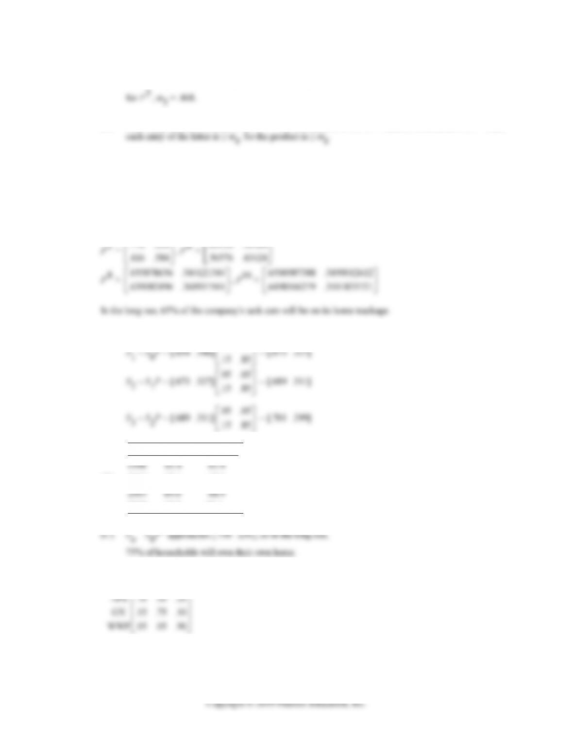
56. The transition matrix is:
H N
P = .86 .14 home trackage
.26 .74 national pool
HH
NN
Calculating powers of P, we have
58. (A) S0 = [.654 .346]
.15 .85
(B)
Year Data (%) Model (%)
2000 67.4 67.3
2008 67.8 70.1
60. The transition matrix for this problem is:
APS GX WWP
APS .70 .10 .20
WWP .05 .05 .90
EXERCISE 15-2 15-15
To find the steady-state matrix, we solve the system
[s1 s2 s3]
.7 .1 .2
.15 .75 .1
.05 .05 .9
= [s1 s2 s3], s1 + s2 + s3 = 1
which is equivalent to the system of equations
.7s1 + .15s2 + .05s3 = s1 –.3s1 + .15s2 + .05s3= 0
Thus, the expected market share of each company is:
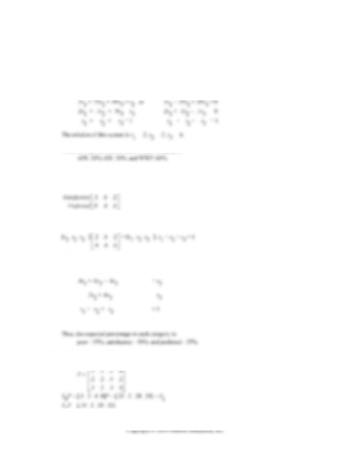
62. The transition matrix for this problem is:
P. Sat. Pref.
.6 .4 0
Poor
To find the steady-state matrix, we solve the system
.6 .4 0
which is equivalent to the system of equations:
.6
s1 + .2s2 = s1
The solution of this system is s1 = .25, s2 = .5, and s3 = .25.
64. The transition matrix is:
.3 .2 .2 .3
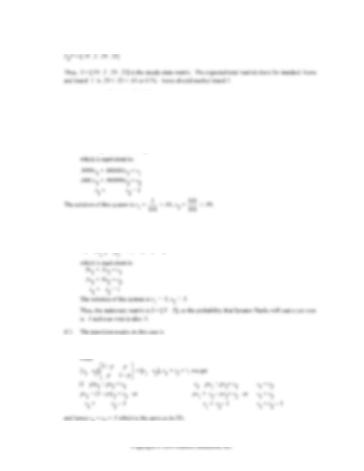
15-16 CHAPTER 15: MARKOV CHAINS
S2P = [.19 .2 .29 .32]
Type A Type B
66. (A) P =
Type .9999 .0001
.000001 .999999
Type
A
B
(B) To find the stationary solution, we solve the system
[s1 s2].9999 .0001
.000001 .999999
= [s1 s2], s1 + s2 = 1,
68. (A) [.1 .9]
(B) To find the stationary solution, we solve the system
[
s1 s2].9 .1
= [s1 s2], s1 + s2 = 1,
P = 1
1
pp
pp
EXERCISE 15-3 15-17
70. (A) S1 = S0P = [0.241 0.759] 0.61 0.39
0.09 0.91
≈ [0.215 0.785];
0.09 0.91
(B)
Year Data (%) Model (%)
1970 24.1 24.1
1990 20.4 20.2
2010 17.9 19.1
(C) P2 ≈ .4072 .5928
, P4 ≈ .24690688 .75309312
,
EXERCISE 15-3
6. No absorbing states. 8. No absorbing states; not an absorbing chain.
10. C and D are absorbing states; the diagram represents an absorbing Markov chain since it is possible to go
12. P = 10
14. P = .6 .4
10
A
B
15-18 CHAPTER 15: MARKOV CHAINS
Copyright © 2019 Pearson Education, Inc.
A B C
16. P =
001
100
B
C
A B C
18. P =
.5 .5 0
.4 .3 .3
A
B
A B C
20. P =
100
001
A
B
22. The transition diagram is represented
by the matrix:
B C A
24. The transition diagram is represented by the matrix
B A C D
1000
B
26. A standard form for
A B C
P =
001
010
A
B
B A C
100
001
.2 .7 .1
B
A
C
28. A standard form for
A B C D
0.3.3.4
0100
A
B
is:
B C A D
1000
0100
B
C
15-20 CHAPTER 15: MARKOV CHAINS
Now A B C
100
A
34. For A B C D
1000
0100
A
B
.3 .1
.4 .2
The limiting matrix P has the form
P =
0
I
01 .4.2
-1
.4 .8
-1
31
10 10
24
55
-1
We use row operations to find the inverse:
3110
10 10
~
10
1
10
33
~
10
1
10
33
~
10
1
10
33
3
0122
Thus, F =
1
2
4
and FR =
1
2
4
.1 .1
= .55 .45
.55 .45 0 0
.65 .35 0 0
C
D
P(C to A) = .55, P(C to B) = .45,