Unlock document.
This document is partially blurred.
Unlock all pages and 1 million more documents.
Get Access
CHAPTER 15
Markov Analysis
TEACHING SUGGESTIONS
Teaching Suggestion 15.1: Use of Matrix Algebra.
Markov analysis requires the use of matrix algebra, primarily matrix multiplication. You may
Module 5.
Teaching Suggestion 15.2: Matrix of Transition.
Markov analysis requires a known and stable matrix of transition. Students should be told that
in the matrix of transition can make a big difference in equilibrium calculations.
Teaching Suggestion 15.3: Application of Markov Analysis.
There are a number of applications of Markov analysis. The applications box in this chapter pre-
Teaching Suggestion 15.4: Sensitivity Analysis and Markov Analysis.
Although sensitivity analysis is not a formal part of the material discussed in this chapter, it is an
Teaching Suggestion 15.5: Equilibrium Conditions and the Beginning State or Condition.
As mentioned in this chapter, equilibrium conditions do not depend on the initial state or condi-
Teaching Suggestion 15.6: Absorbing State Analysis and Matrix Algebra.
Absorbing state analysis requires more complex matrix algebra, including the inverse of the (I − B)
ALTERNATIVE EXAMPLES
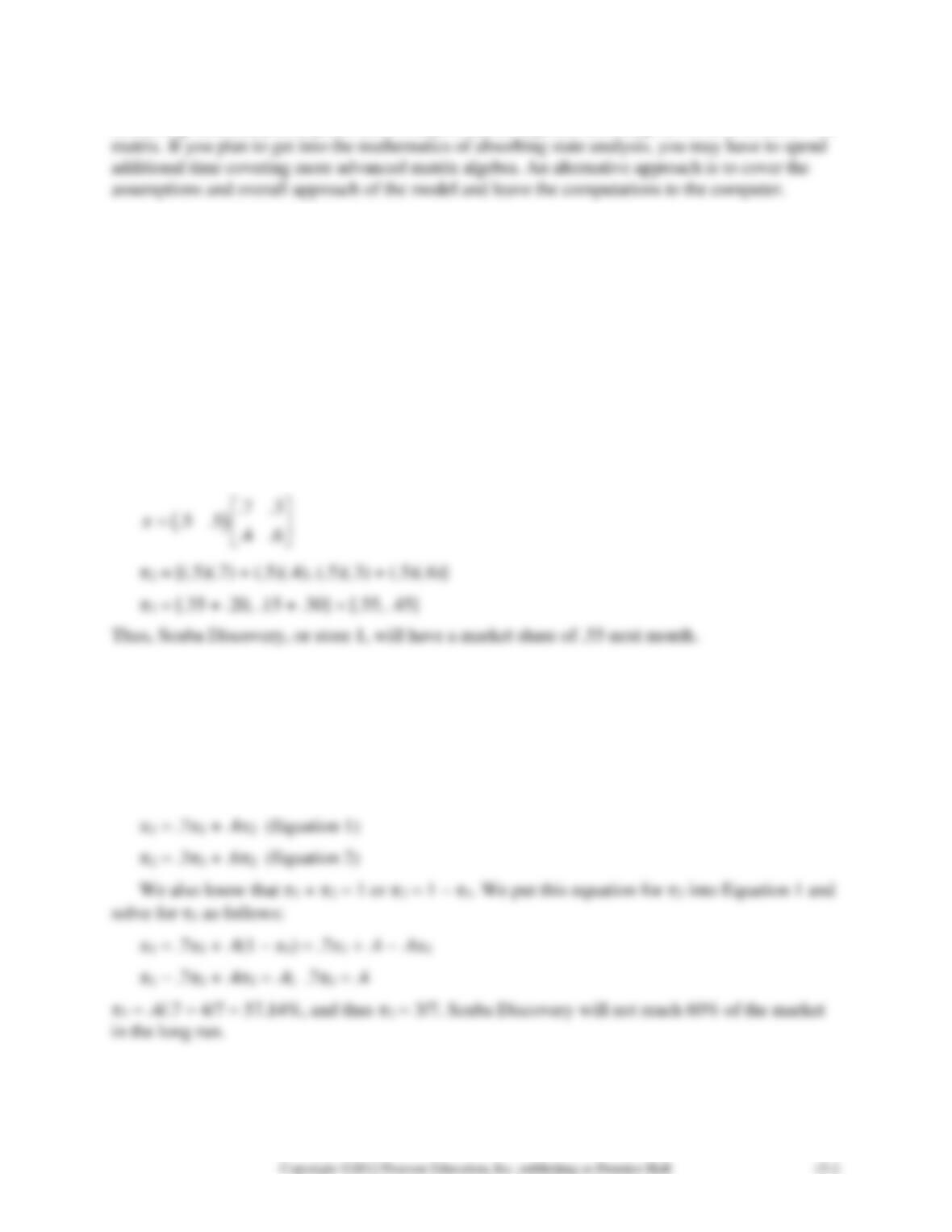
Alternative Example 15.1: Scuba Discovery (Store 1) currently splits the market for scuba
classes with Bob’s Dive Shop. Given the matrix of transition probabilities below, what will the
market shares be next month (period)?
.7 .3
.4 .6
P
=
We start by noting that the initial state or 1 is (.5 .5) or equal shares of the market. We can de-
termine the market shares for next month or 2 as follows:
2 = 1P
Alternative Example 15.2: Scuba Discovery would like to determine its equilibrium market
share. (See Alternate Example 15-1.) Will the store eventually capture 60% of the market in the
long run?
To solve this problem, we set up the equilibrium equations and solve for 1 and 2. The re-
sults are below:
SOLUTIONS TO DISCUSSION QUESTIONS AND PROBLEMS
15-1. Markov analysis makes the assumption that the propensity to change over time stays the
same. This tendency to change is embodied in the matrix of transition. Furthermore, it is as-
15-2. The vector of state probabilities is a collection of probability values that the particular sys-
tem will be in a given state. In most cases it is determined using historical data. For example, if
15-3. Future states can be determined by multiplying the current state probabilities by the matrix
of transition. If we want to determine future market shares in August, we multiply the market
shares in July by the matrix of transition. This process can be repeated to determine future states
several months or years in the future.
15-4. An equilibrium condition is a condition in which the state probabilities do not change from
one period to the next. We can compute the equilibrium conditions by setting the unknown equi-
15-5. An absorbing state is one in which once it is entered, it cannot be left. In the matrix of
15-6. The fundamental matrix is equal to the inverse of the identity matrix minus the B matrix.
The B matrix is determined by partitioning the matrix of transition. The fundamental matrix is
then multiplied by the A matrix, which is another partition of the matrix of transition.
15-7.
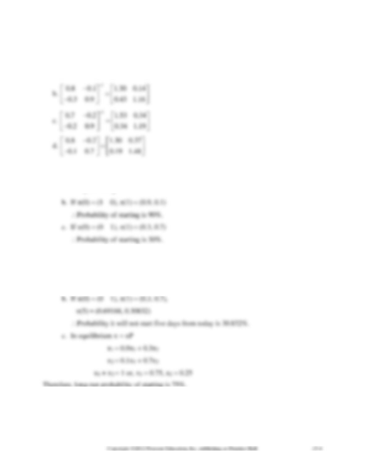
a.
1
0.9 0.1 1.15 0.16
0.2 0.7 0.33 1.48
−
−
=
−
15-8. State 1: start; state 2: not start
a.
0.9 0.1
0.3 0.7
P
=
15-9. a. If (0) = (1 0), (1) = (0.9, 0.1),
(5) = (0.76944, 0.23056)
Probability it will not start five days from today is 23.056%.
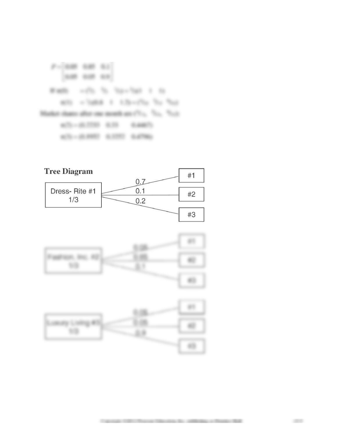
15-10. If states 1, 2, and 3 represent Dress-Rite, Fashion, Inc., and Luxury living customers:
0.7 0.1 0.2
After three months, market shares will be 19.52%, 32.52%, and 47.96%.
15-11.
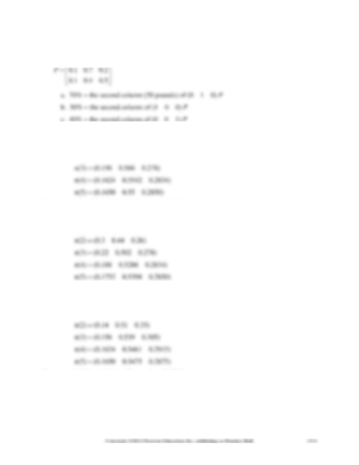
15-12. Let states 1, 2, 3 correspond to placing 49, 50, and 51 pounds into the bags. Then
0.5 0.3 0.2
15-13. a. If (0) = (0 1 0)
(1) = (0.1 0.7 0.2),
(2) = (0.14 0.6 0.26)
Therefore probability of placing 50 pounds is 55%.
b. If (0) = (1 0 0)
(1) = (0.5 0.3 0.2)
Required probability of placing 50 pounds is 53.98%.
c. If (0) = (0 0 1)
(1) = (0.1 0.4 0.5)
Hence, probability of placing 50 pounds = 54.75%.
15-14.
0.6 0.2 0.1 0.1
0.0 0.7 0.2 0.1
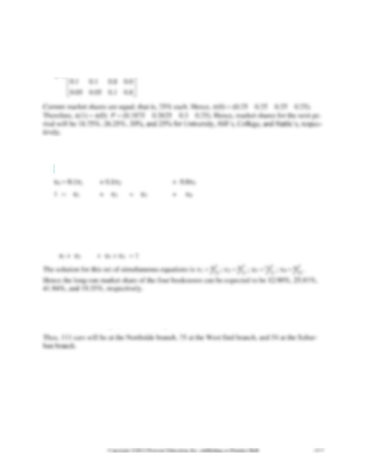
15-15. In the long run, = P. We drop the equation for 2 and solve.
1 = 0.61 + 0.13 + 0.054
3 = 0.11 + 0.22 + 0.83 + 0.14
which simplify to:
−81 + 23 + 4 = 0
1 + 22 − 23 + 4 = 0
1 + 2 −24 = 0
15-16.
0.80 0.10 0.10
100 80 60 0.20 0.70 0.10 111 75 54
0.25 0.15 0.60
=
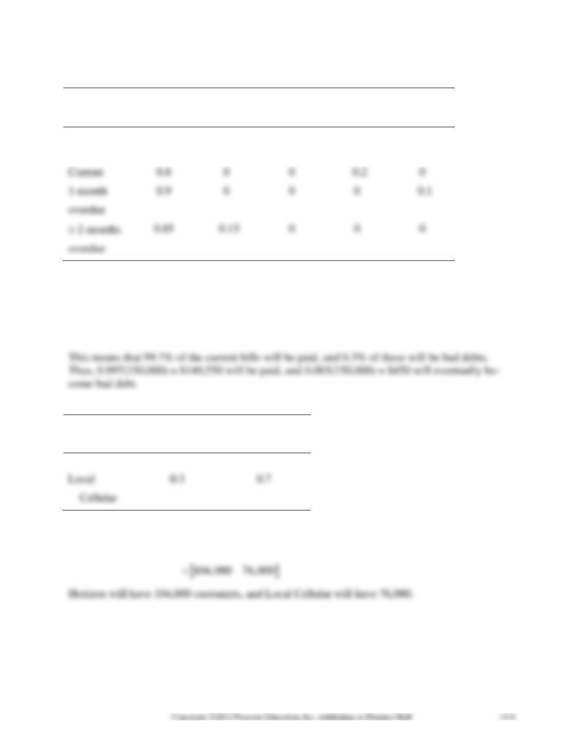
15-17. The matrix of transition probabilities is:
1-month
2-months
Paid
Bad Debt
Current
overdue
overdue
Paid
1
0
0
0
0
Bad Debt
0
1
0
0
0
Using QM for Windows, we have
0.997 0.003
FA= 0.985 0.015
0.850 0.150
15-18. The matrix of transition probabilities is
Local
Horizon
Cellular
Horizon
0.8
0.2
Market shares next year =
0.8 0.2
100,000 80,000 0.3 0.7
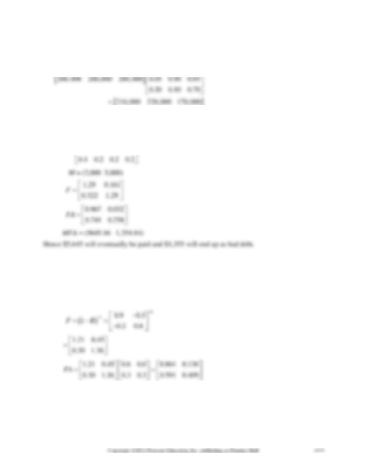
15-19. Next year, Doorway will sell 210,000, Bell will sell 220,000, and Kumpaq will sell
170,000.
0.80 0.10 0.10
15-20.
1 0 0 0
0 1 0 0
0.7 0 0.2 0.1
P
=
15-21.
1 0 0 0
0 1 0 0
0.6 0 0.1 0.3
0.3 0.3 0.2 0.2
P
=
If M = (50 30)
( ) ( )
0.864 0.136
50 30 61 19
0.591 0.409
MGA
==
Hence, 61 will pass and 19 fail the course.
15-22. The Hicourt Industries problem requires some careful thought and analysis. At first
glance, it appears that there is insufficient data to solve the problem. Important matrix of transi-
tion values are seemingly missing. For this particular problem, we will assume that Hicourt In-
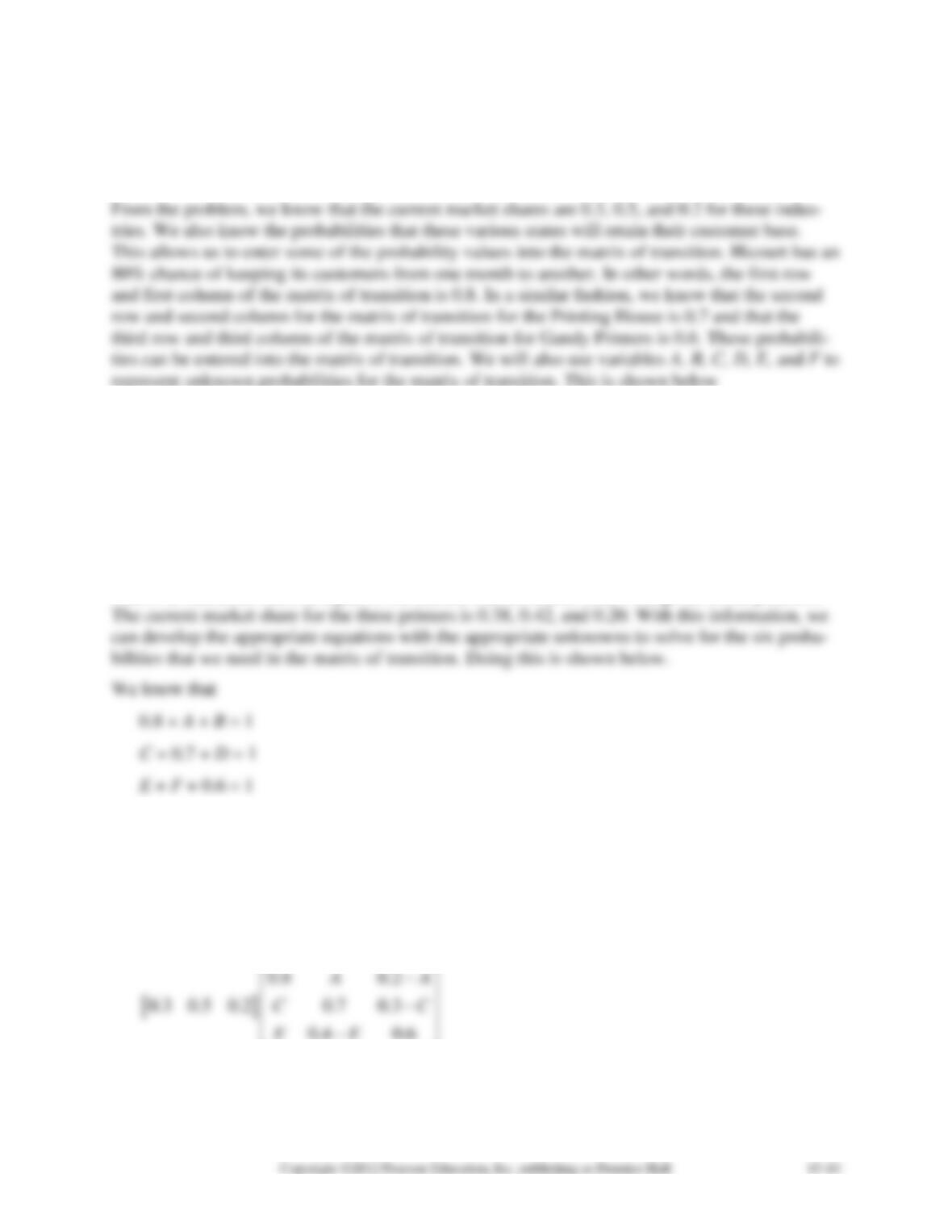
dustries will be state 1, the Printing House will be state 2, and Gandy Printers will be state 3.
0.8
0.3 0.5 0.2 0.7
0.6
AB
CD
EF
Before we can go any further, we must determine a value for the six unknown probabilities in
the matrix of transition. As seen above, these probabilities have been represented by the varia-
bles, A, B, C, D, E, and F. To begin with, we know that the probabilities for any row in the ma-
trix of transition must sum to one. We also know that the original market shares multiplied by the
matrix of transition must be equal to the current market share, which was given in the problem.
or
B = 0.2 − A
D = 0.3 − C
F = 0.4 − E
Putting these into the matrix of transition, we get
0.4 0.6
EE
−
= [0.38 0.42 0.20]
Since we know that the matrix of transition probabilities multiplied by a previous market
share is equal to a future market share, we can solve the problem above and get three equations
and three unknowns. These equations can be solved for A, C, and E. These values can then be
substituted into previous equations to determine values for B, D, and F. This will completely
specify our matrix of transition probabilities. This is shown below.
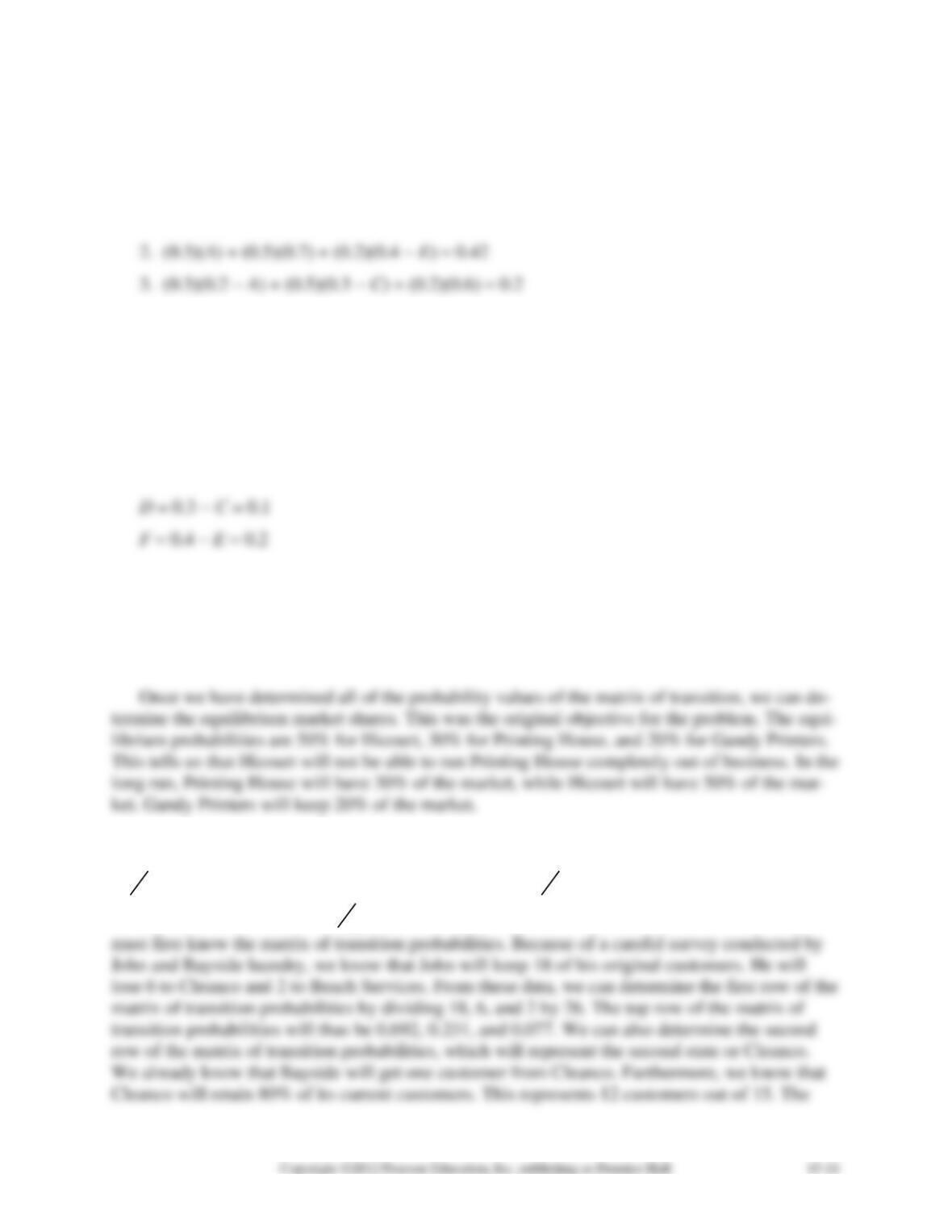
1. (0.3)(0.8) + (0.5)(C) + (0.2)E = 0.38
Solving the above, we get
A = 0.1
C = 0.2
E = 0.2
From this we can compute B, D, and F:
B = 0.2 − A = 0.1
Thus the matrix of transition is:
0.8 0.1 0.1
0.2 0.7 0.1
0.2 0.2 0.6
15-23. For John to get the loan that he desires, he must keep at least 35% of the market share in
the long run. Currently, John has 26 condominiums, representing 50% of the market (0.50
=
2652
). Cleanco has about 28.8% of the market (0.288 =
1552
) and Beach Services has about
21.2% of the market (0.212 =
1152
). In order for us to determine equilibrium market shares, we
remaining 2 customers out of the original 15, therefore, must have switched to Beach Services.
By dividing the numbers 1, 12, and 2 by 15, we know the second row of the matrix of transition
probabilities. Doing this will give us 0.067, 0.80, and 0.133 for the second row of the matrix of
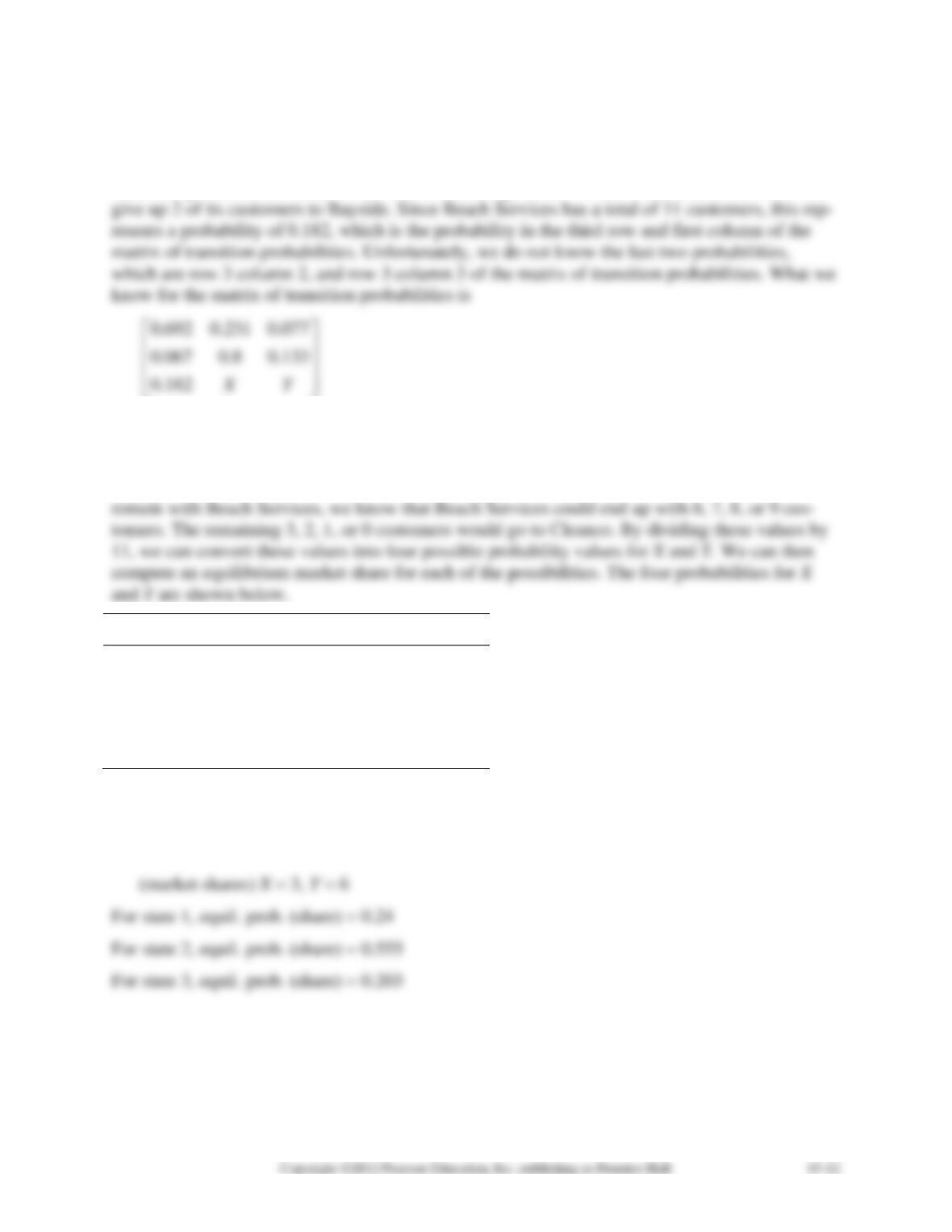
transition probabilities. Here, we run into a stumbling block. We know that Beach Services will
As you can see, all of the probabilities are known but the last two in the third row. These are
represented by the variables X and Y. It was also given in the problem that Beach service would
keep at least 50% of its current customers. Fifty percent of the current customers would be 6 cus-
tomers. Since we know that 2 customers are going to Beach Services and at least 6 customers
X
Y
P(X)
P(Y)
3
6
0.273
0.545
2
7
0.182
0.636
1
8
0.091
0.727
0
9
0
0.818
From the probability values above, we can determine the equilibrium market share for each
possibility. The results are shown below.
Equilibrium state probabilities
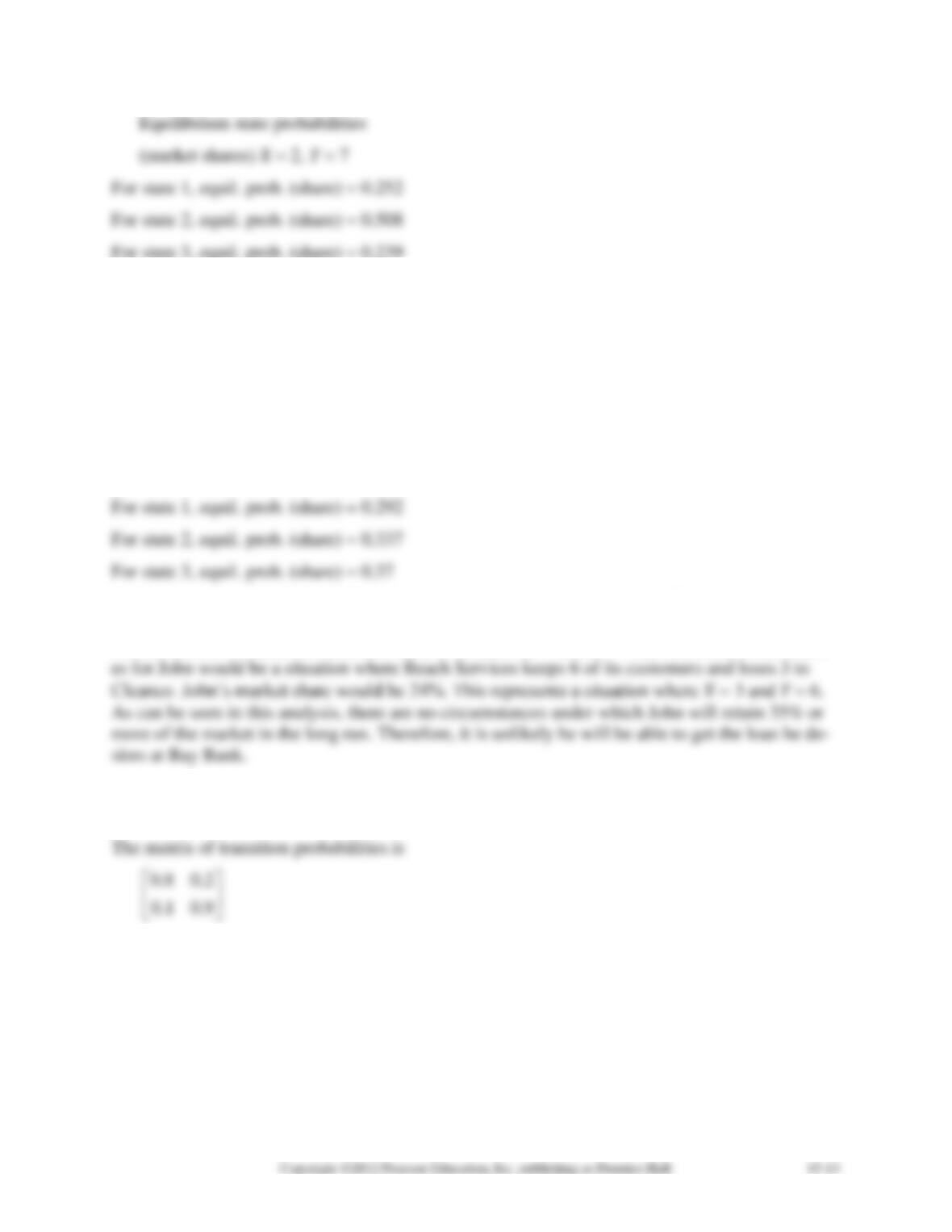
Equilibrium state probabilities
(market shares) X = 1, Y = 8
For state 1, equil. prob. (share) = 0.267
For state 2, equil. prob. (share) = 0.441
For state 3, equil. prob. (share) = 0.29
Equilibrium state probabilities
(market shares) X = 0, Y = 9
As you can see from the analysis, the highest market share that John will achieve would be
approximately 29.2% of the market in the long run. This assumes that Beach Services will retain
9 of its current 11 customers and lose none to Cleanco (X = 0 and Y = 9). The worst circumstanc-
15-24. The vector of state probabilities is
(0.40, 0.60)
15-25. (2) = (0.38, 0.62).
15-26.
1
1
3
=
;
2
2
3
=
. Given no changes in the Markov assumptions, store 1 will eventually
end up with one-third of the customers, while store 2 will end up with two-thirds of the custom-
ers.
3
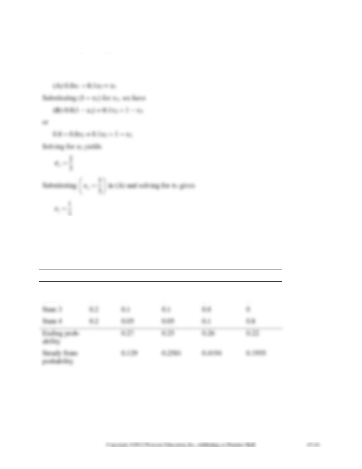
15-27. This problem can be solved using QM for Windows. The results are presented below. As
you can see from the ending probabilities, the market shares change for the next period. The
market shares for University, Bill’s, College, and Battle’s stores are 27%, 25%, 26%, and 22%.
The steady-state market shares do not change, as you would expect.
Data
Initial
State 1
State 2
State 3
State 4
State 1
0.4
0.6
0.2
0.1
0.1
State 2
0.2
0
0.7
0.2
0.1


