Chapter 14
Inventory Models
Case Problem 1: Wagner Fabricating Company
1. Holding Cost
Cost of capital 14.0%
Taxes/Insurance (24,000/600,000) 4.0%
2. Ordering Cost
2 hours at $28.00 $56.00
Other expenses (2,375/125) 19.00
Cost per order $75.00
4. & 5.
a. Order from Supplier – EOQ model
Number of orders = D/Q = 9.19/year
Cycle time = 250(Q) / D = 250(348.16) / 3200 = 27.2 days
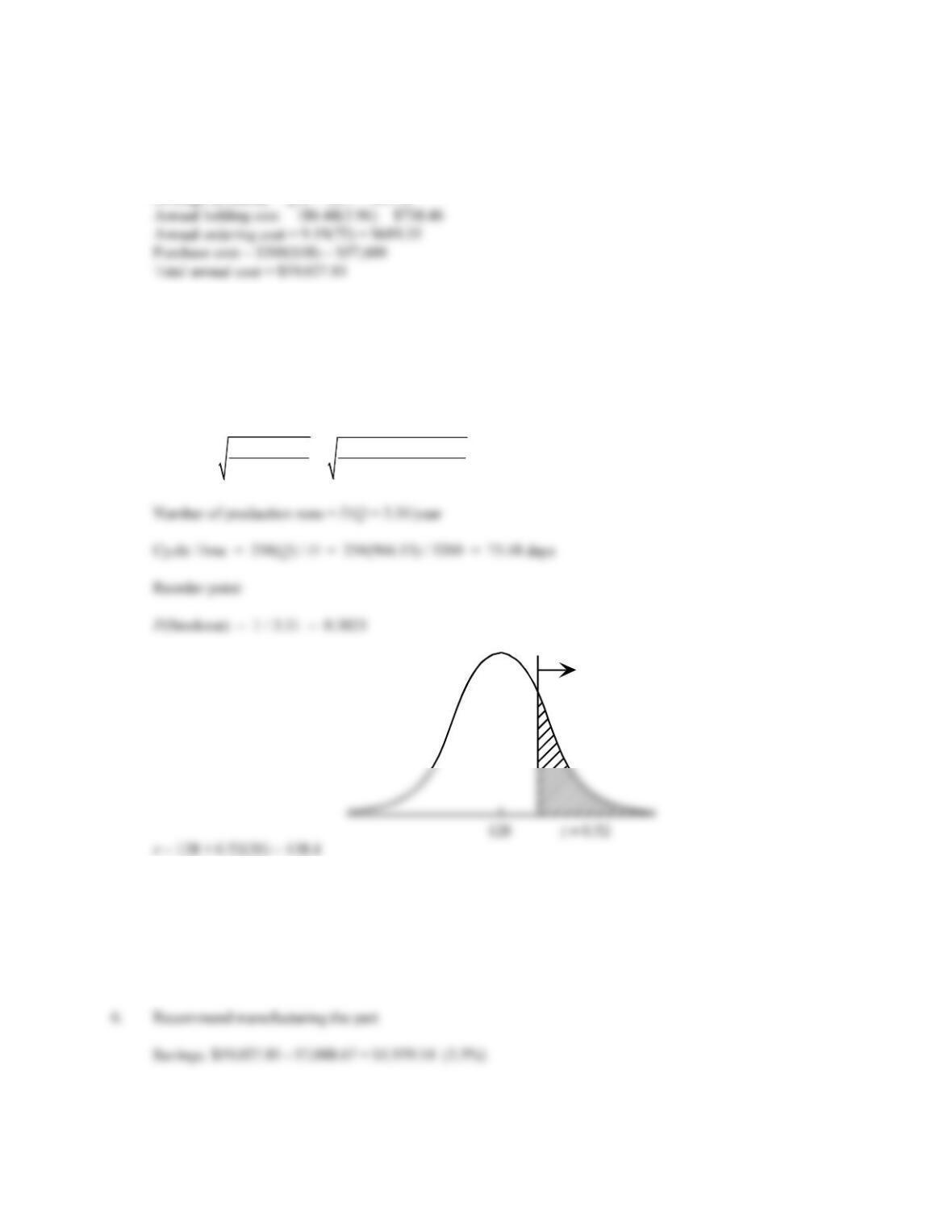
Reorder Point:
P(Stockout) = 1 / 9.19 = 0.1088
Chapter 14
14 –
2
r = 64 + 1.24(10) = 76.4
Safety stock = 76.4 – 64 = 12.4
Maximum inventory = Q + 12.4 = 360.56
b. Manufacture – Production lot size model
Ch = IC = 0.22($17.00) = $3.74
P = 1000(12) = 12,000/year
Note: The five-month capacity of 5,000 units is sufficient to handle annual demand of 3,200 units.
22(3200)(400)
* 966.13
(1 / ) (1 3200/1200)3.74
o
h
DC
QD P C
= = =
−−
Safety stock = 138.4 – 128 = 10.4
Maximum inventory = (1 – 3200/12000)966.13 + 10.4 = 718.89
Annual holding cost = (354.25 + 10.4)(3.74) = $1363.79
Annual set up cost = 3.31(400) = $1363.79
Manufacturing cost = 3200($17) = $54,400
Total Annual Cost = $57,088.67
Stockout
14 –
3
Case Problem 2: River City Fire Department
1. During a three-week scheduling period, a unit is scheduled seven days and must have at least 186 firefighters
on duty each day. Thus, each unit must provide staffing for
7
186 = 1302 firefighter days
2. The single-period inventory model can be used to determine the number of additional firefighters to be added
to the unit to cover daily absences.
Let Q* = minimum cost number of additional firefighters
If Demand < Q*, Q* has overestimated demand.
cu = 1.55d – d = 0.55d
Using the single period inventory model,
0.55 0.55
(Demand *) 0.3548
0.55 1.55
u
uo
cd
PQ
c c d
= = = =
++
Using the normal distribution, area = 0.5000 – 0.3548 = 0.1452. z = -0.37
Chapter 14
14 –
4
3. From part 2, this is the probability demand will exceed 18.14 is 1 – 0.3548 = 0.6452. This is an acceptable
approximation of the probability overtime will be needed.
4. Firefighters for each unit
217 + 18 additional = 235
17 – 1