CHAPTER 14
Simulation Modeling
TEACHING SUGGESTIONS
Teaching Suggestion 14.1: There Are Many Kinds of Simulations.
This chapter teaches the concepts of Monte Carlo simulation, but it also notes that there are
Teaching Suggestion 14.2: Examples of Advantages of Simulation.
Section 14–2 lists 8 advantages of simulation. Have students provide an example of numbers 3, 4,
6, 7, and 8 in order to be sure these points are made. Hospitals are especially good cases for
number 5—“do not interfere with the real–world system.”
Teaching Suggestion 14.3: Use of the Cumulative Probability Distribution in Setting Random
Number Intervals.
Teaching Suggestion 14.4: Starting the Random Number Intervals at 01 or 00.
Teaching Suggestion 14.5: Another Way to Generate Random Numbers.
Excel and other spreadsheets make simulation a quick and relatively painless process compared
to other methods.
Teaching Suggestion 14.6: Use of Computers for Speedy Simulations.
Teaching Suggestion 14.7: Relating Simulation to the Inventory Chapter.
Students should start to see the relationship between simulation and most of the other techniques
in the book. Because of all the EOQ limiting assumptions, simulation is an important tool.
Teaching Suggestion 14.8: Gaming in Business Courses.
Teaching Suggestion 14.9: Outside Research Articles.
This is a good chapter for students to find down-to-earth published articles on a wide variety of
ALTERNATIVE EXAMPLES
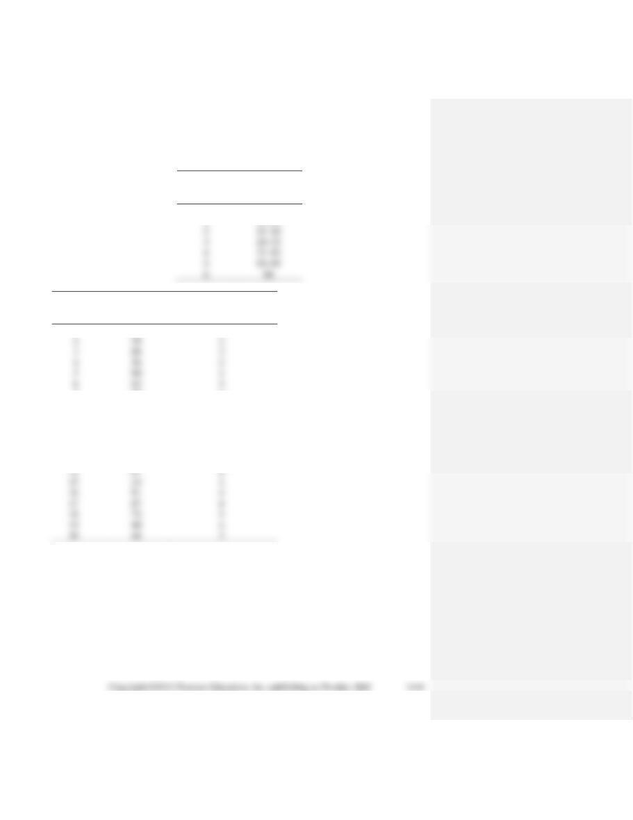
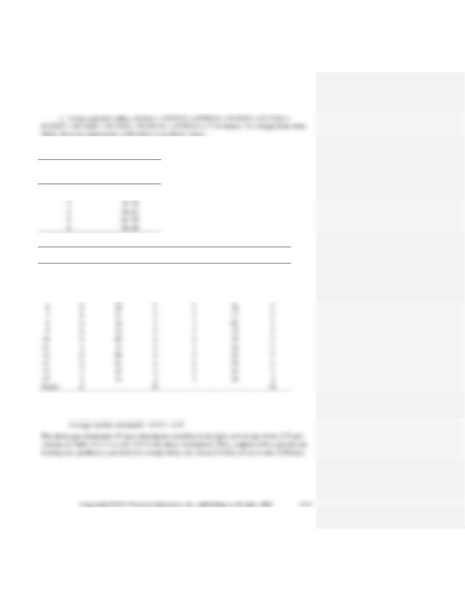
Alternative Example 14.1: The number of cars arriving at a self-service gasoline station during
the last 50 hours of operation are as follows:
Number of Cars Arriving
Frequency
6
10
7
12
8
20
9
The following random numbers have been generated: 44, 30, 26, 09, 49, 13, 33, 89, 13, 37. Sim-
ulate 10 hours of arrivals at this station. What is the average number of arrivals during this peri-
od?
SOLUTION:
Number of Cars
RN
6
01–20
7
21–44
8
45–84
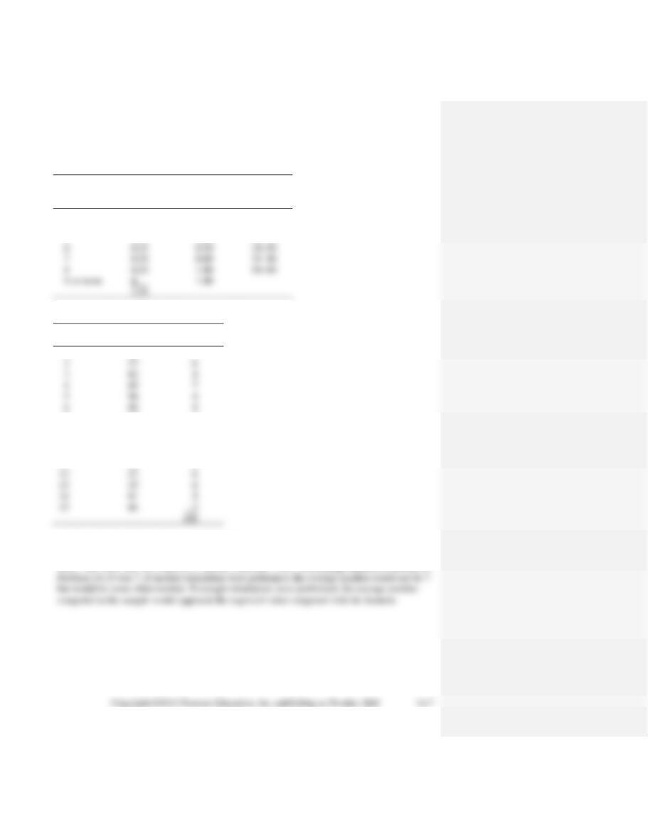
Alternative Example 14.2: Average daily sales of a product are 8 units. The actual number of
sales each day is 7, 8, or 9 with probabilities 0.3, 0.4, and 0.3, respectively. The lead time for de-
livery averages 4 days, although the time may be 3, 4, or 5 days with probabilities 0.2, 0.6, and
0.2. The company plans to place an order when the inventory level drops to 32 units (based on
the average demand and average lead time).
SOLUTION:
Sales
RN
Lead Time
RN
7
01–30
3
01–20
8
31–70
4
21–80
9
71–00
5
81–00
First order: RN = 60 so lead time = 4 days.
Demand day 1 8 (RN = 52)
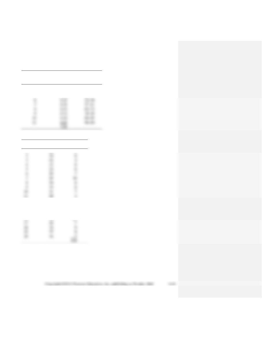
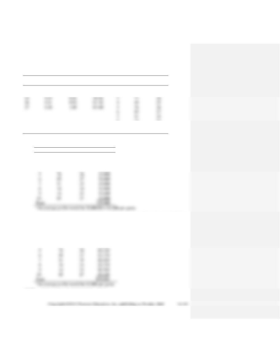
Alternative Example 14.3: The time between arrivals at a drive-through window of a fast-food
restaurant follows the distribution given below. The service time distribution is also given in the
table in the right column. Use the random numbers provided to simulate the activity of the first
five arrivals. Assume that the window opens at 11:00 A.M. and the first arrival is after this, based
on the first interarrival time generated.
Time
Between
Service
Arrivals
Probability
Time
Probability
1
0.2
1
0.3
2
0.3
2
0.5
3
0.3
3
0.2
SOLUTION:
Time
Between
Service
Arrivals
Prob.
RN
Time
Prob.
RN
1
0.2
01–20
1
0.3
01–30
2
0.3
21–50
2
0.5
31–80
SOLUTIONS TO DISCUSSION QUESTIONS AND PROBLEMS
14–1. Advantages of simulation: (1) relatively straightforward; (2) software advanbces makes it
easy; (3) can solve large, complex problems; (4) allows “what if” questions; (5) does not inter-
14–2. a. Inventory ordering policy: May require simulation if lead time and daily demand are not
constant. Also useful if data do not follow a traditional probability distribution.
b. Ships docking in port to unload: If arrivals and unloadings do not follow Pois-
son/exponential distributions common to queuing problems, or if other queuing model assump-
tions are violated (for example, FIFO not observed).
14–3. Problems with conditions of certainty can be solved more easily by other QA techniques.
Problems that require quick answers that cannot wait for a simulation model to be built are a
second category.
14-4. Major steps are: (1) define problem, (2) introduce important variables, (3) construct mod-
el, specify values to test, (4) conduct simulation, (5) examine results, (6) select best plan.
14–6. Random numbers can be generated by: (1) computer programs such as Excel, (2) spinning
a dial on a uniform wheel, (3) pulling numbers from an urn, (4) using a random number table,
and (5) creating an algorithm such as the midsquare method.
14–9. The results would very likely change, and perhaps significantly, if a longer period was
simulated. The 10-day simulation is valid only to illustrate the features of the system. It would
not be safe to forecast based on that short a span.
14–10. A computer is necessary for three reasons: (1) it can do time periods or trials in a matter
of seconds or minutes, (2) it can quickly examine and allow change in the complex interrelation-
ships being studied, and (3) it can internally (through a subroutine or function statement) gener-
ate random numbers by the thousands or millions.
14–11. Operational gaming is a simulation involving competing players. Systems simulation
tests the operating environment of a large system such as a corporation, government, or hospital.
14–14.
Random
Number of
Number
Failures
Interval
0
01–06
1
07–19
6
Number of A.C.
Simulated
Random
Compressors Simulated
Period
Number
to Fail This Year
1
50
3
2
28
2
68
3
36
2
90
4
62
3
7
27
2
8
50
3
9
18
1
10
36
2
11
61
3
12
21
2
13
46
3
14
01
0
15
14
1
81
4
17
87
4
18
72
3
19
80
4
20
46
3
No, it’s not common to find three or more years in a row with two or less compressor failures.
14–15. a, b. Lundberg’s car wash:
Random
Number of
Cumulative
Number
Cars
Probability
Probability
Interval
3 or less
0
0.00
—
4
0.10
0.10
01–10
5
0.15
0.25
11–25
6
0.25
0.50
26–50
8
0.20
1.00
81–00
9 or more
0.
1.00
—
c.
Random
Simulated
Hour
Number
Arrivals
1
52
7
37
6
3
82
8
4
69
7
5
98
8
6
96
8
7
33
6
8
50
6
9
88
8
10
90
8
11
50
6
12
27
6
13
45
6
81
8
66
Average number arrivals per hour = 105/15 = 7 cars.
14–16. Using the probability distribution developed in Problem 14-15, the expected value is
E(X) = 4(0.10) + 5(0.15) + 6(0.25) + 7(0.30) + 8(0.20) = 6.35. The average number of arrivals in
14–17. Higgins plumbing:
Random
Number
Heater Sales
Probability
Intervals
3
0.02
01–02
4
0.09
03–11
5
0.10
12–21
6
0.15
22–36
8
0.12
62–73
9
0.12
74–85
0.05
96–00
1.00
a.
Random
Simulated
Week
Number
Sales
24
6
03
4
32
6
23
6
59
7
95
10
12
48
7
13
66
8
14
97
11
15
03
4
16
96
11
20
44
With a supply of 8 heaters, Higgins will stock out 5 times during the 20-week period (in weeks 7,
14, 16, 18, and 19).
b. Average sales by simulation = total sales/20 weeks = 139/20 = 6.95. Other simula-
tions by students will yield slightly different results.
14–18. a.
New
Random Number
Unloading Rate
Interval
1
01–03
2
04–15
4
56–83
Table for Problem 14-18
Number
Random
Daily
Total to Be
Random
Number
Day
Delayed
Number
Arrivals
Unloaded
Number
Unloaded
1
—
37
2
2
69
2
2
0
77
4
4
84
4
3
0
13
0
0
12
0
4
0
10
0
0
94
0
5
0
02
0
0
51
0
6
0
18
1
1
36
1
1
31
2
3
16
3
0
94
5
5
52
3
2
81
4
6
56
4
2
43
2
4
43
3
1
31
3
26
3
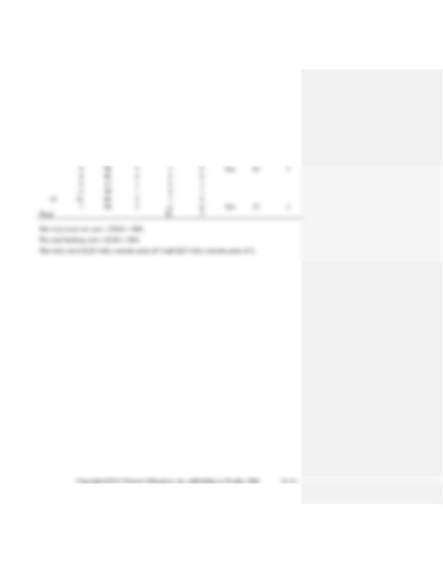
b. Average number delayed = 6/15 = 0.40
Average number of arrivals = 31/15 = 2.07
14–19. a
Interval
Demand
X
P(X)
Cum. Prob.
of RN
Day
RN
(100s)
23
0.15
0.15
1–15
1
07
23
24
0.22
0.37
16–37
2
60
25
25
0.24
0.61
38–61
3
77
26
8
16
24
9
14
23
10
85
27
b. If 25 hundred programs are printed, the maximum number sold will be 2,500. Thus, the
profits are $2 per program sold less the cost of printing 2,500.
Day
RN
Demand
Profit
1
07
23
$2,600
2
60
25
$3,000
3
77
26
$3,000
4
49
25
$3,000
9
14
23
$2,600
85
27
Total
c. If 26 hundred were printed, the profits are $2 per program sold less the cost of printing
2,600.
Day
RN
Demand
Profit
1
07
23
$2,520
2
60
25
$2,920
3
77
26
$3,120
4
49
25
$2,920
5
76
26
$3,120
85
27
Total
14–20. a. Using column 4 of Table 14.4 we have

RN
Probability
Interval
Weather
Day
RN
Weather
0.8
1–80
Good
1
88
Bad
0.2
81–00
Bad
2
02
Good
3
28
Good
4
Good
b.
Interval
P(X)
Cum. Prob.
of RN
Sales
Day
RN
Demand
0.25
0.25
1–25
12
1
53
14
0.24
0.49
26–49
13
2
74
15
0.19
0.68
50–68
14
3
05
12
0.17
0.85
69–85
15
4
71
15
0.15
1.00
86–00
16
5
12
69
15
c.
d. There are several ways that this simulation can be performed. We first simulate the
weather, and we will use the results from part b to get this. We will then use the random
Game
Weather
RN for demand
Demand
Profit
1
Bad
52
14
800
2
Good
37
24
2800
3
Good
82
26
3000
4
Good
69
26
3000
7
Good
33
24
2800
9
Good
88
27
3000
90
27
Total profits = $23,400
14–21. We will use the following random number intervals when simulating demand and lead
time. We will select column 1 to get the random numbers for demand, while we will use column
2 to find the lead time whenever an order is placed.
Cumulative
RN
Probability
Probability
Interval
Demand
0.20
0.20
1–20
0
0.40
0.60
21–60
1
0.20
0.80
61–80
2
0.05
1.00
96–00
4
Cumulative
RN
Lead
Probability
Probability
Interval
Time
0.35
0.50
16–50
2
The results are:
Units
Begin
Lost
Lead
received
Inv.
RN
Demand
End Inv.
Sales
Order?
RN
time
5
52
1
4
0
4
37
1
3
0
3
82
3
0
0
Yes
06
1
0
69
2
0
2
Total
5
The total stock out cost = 5($40) = $200.
The total holding cost = 23($1) = $23.
14–22. If the reorder point Problem 14–21 is changed to 4 units, we have:
Units
Begin
Lost
Lead
received
Inv.
RN
Demand
End Inv.
Sales
Order?
RN
time
5
52
1
4
0
Yes
6
1
4
37
1
3
0
10
13
82
3
10
0
10
69
2
8
0
4
96
4
0
0
0
33
1
0
1
88
3
7
0
7
90
3
0
Yes
57
3
Total
40
2

14-23. Q = 12 drills; reorder point = 6 drills. Using last column of Table 14.4
Lead
Units
Beginning
Random
End
Lost
Random
Time
Day
Received
Inventory
Number
Demand
Inventory
Sales
Order?
Number
(Days)
1
—
12
07
1
11
0
No
2
0
11
60
3
8
0
No
3
0
8
77
4
4
0
Yes
49
2
4
0
4
76
4
0
0
No
5
0
0
95
5
0
5
No
6
12
51
3
9
0
No
7
0
9
16
2
7
0
No
8
0
7
14
1
6
0
Yes
85
3
9
0
6
59
3
3
0
No
0
3
85
4
1
No
Totals
48
6
Random numbers will differ from student to student. Ours were selected from the right-hand column of Table 14.5.
Daily order cost = ($10)(0.2 order/day)
= $2.00
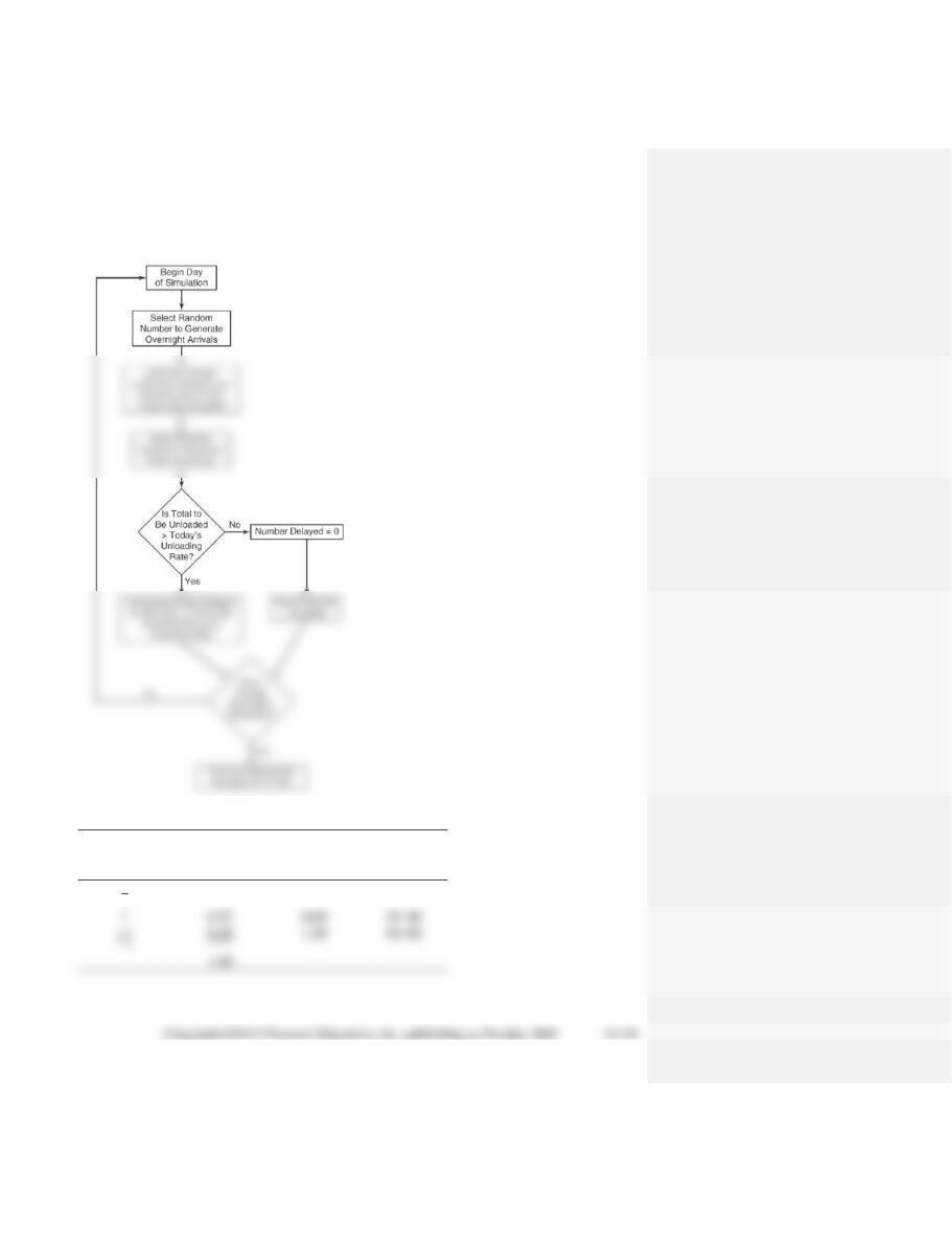
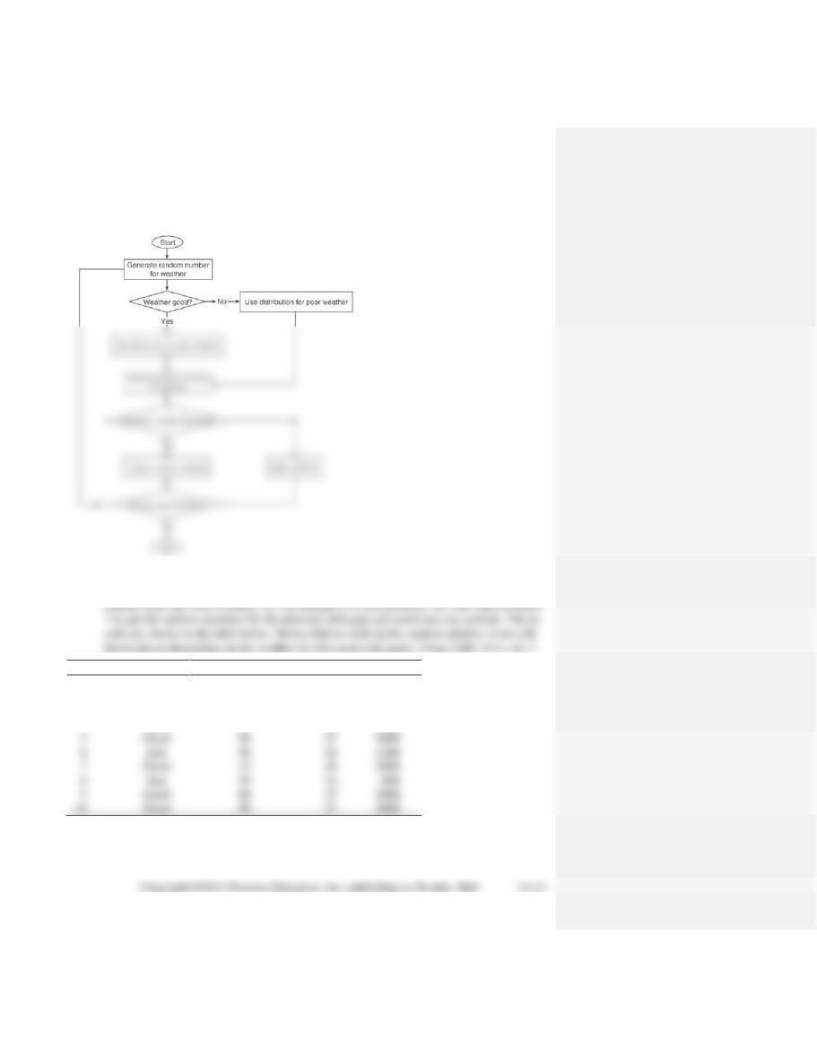
14–24. Flow diagram for Port of New Orleans simulation:
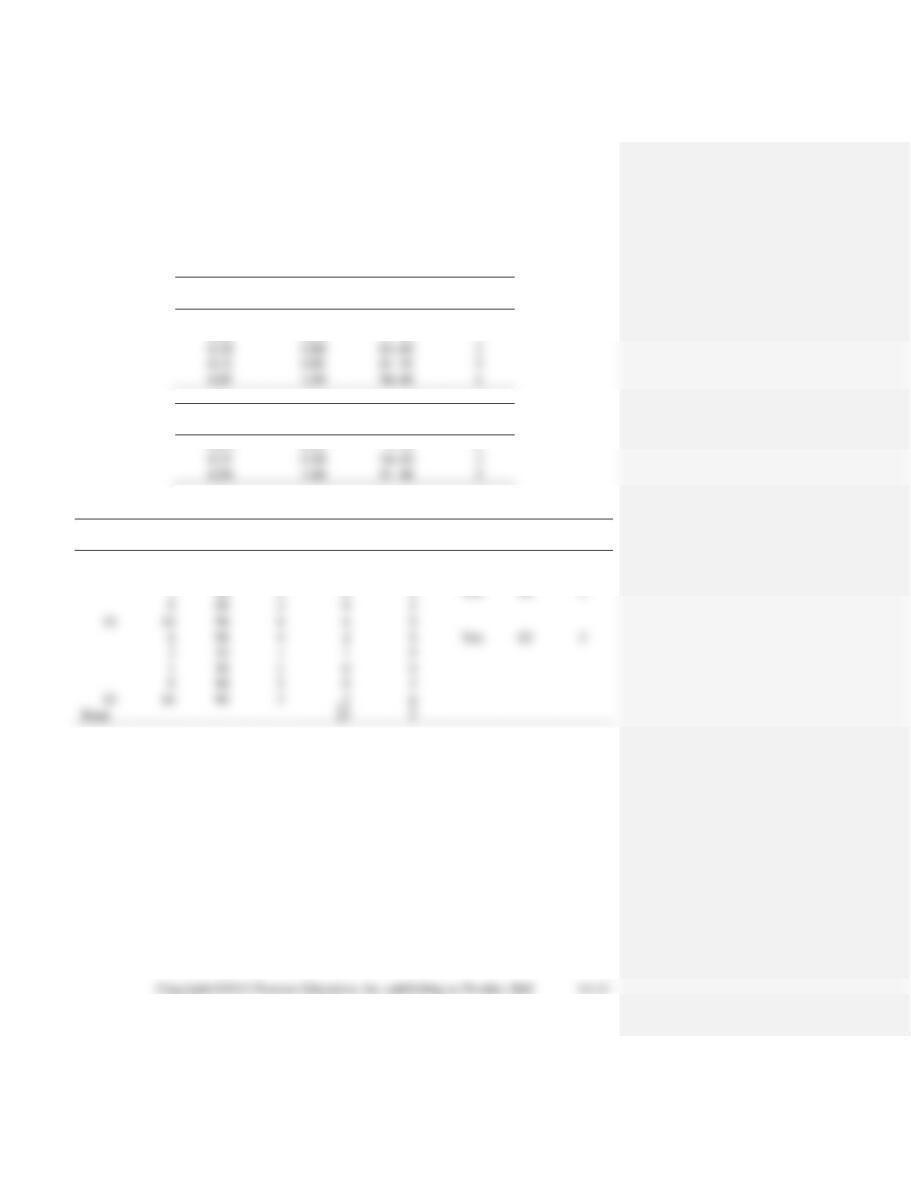
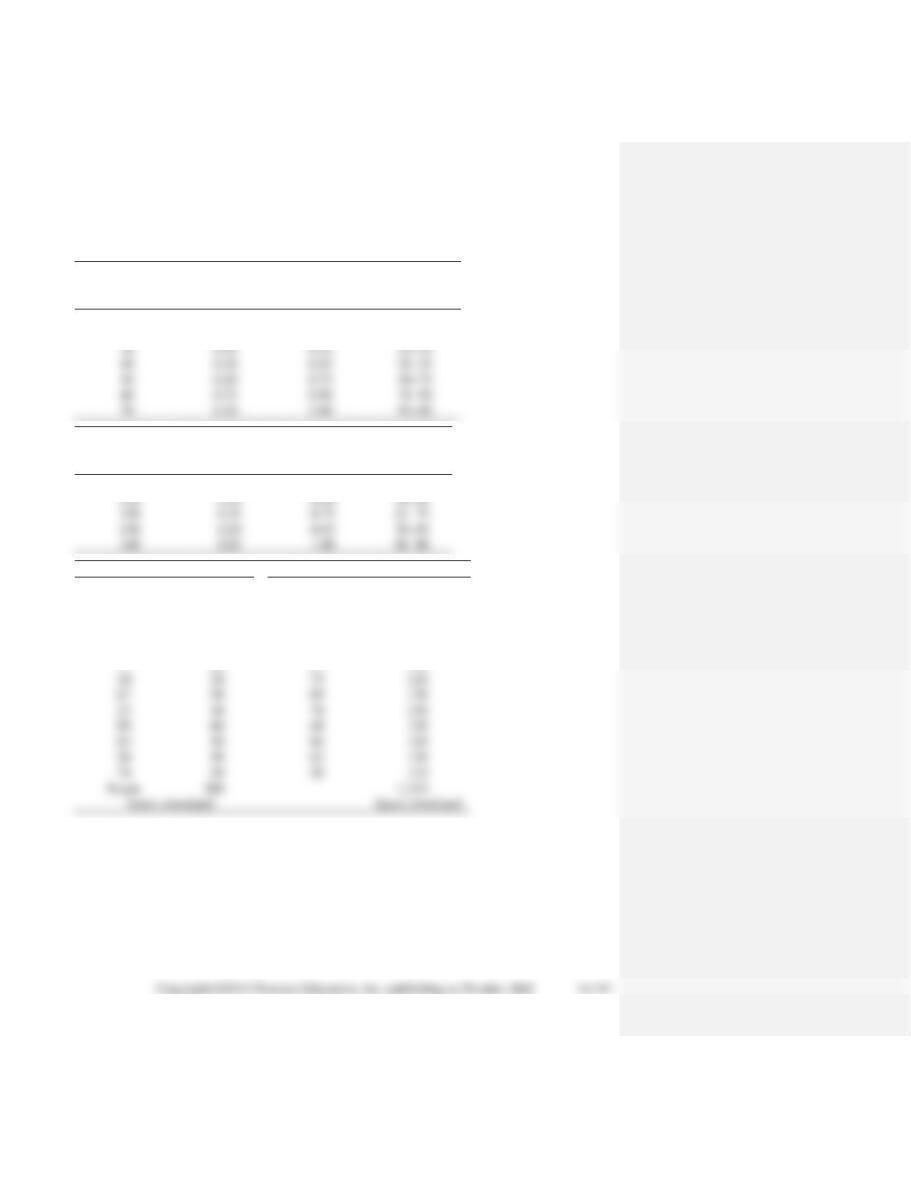
14–25. a. Repair time required with two-person crews:
Repair Time
Random
Required
Cumulative
Number
(Hours)
Probability
Probability
Interval
1
2
1
2
0.28
0.28
01–28

Time
Time
Repair-
Between
Person
Repair
Break-
Break-
Time of
is Free
Time
Time
No. Hours
down
Random
down
Break-
to Begin
Random
Required
Repair
Machine
Number
Number
(Hours)
down
This Repair
Number
(Hours)
Ends
Down
1
69
2
1
2
02:30
02:30
37
1
03:30
1
2
84
3
05:30
05:30
77
1
06:30
1
3
12
2
2
2
1
2
1
2
5
51
2
12:00
12:00
02
1
2
12:30
1
2
1
1
1
07:00
07:00
13
1
07:30
1
2
2
7
17
1
1
2
15:30
15:30
31
1
16:30
1
8
02
1
2
16:00
16:30
19
1
2
17:00
1
9
15
1
1
2
17:30
17:30
32
1
18:30
1
10
29
2
19:30
19:30
85
1
2
2
16
1
2
21:00
21:00
31
1
22:00
1
52
2
23:00
23:00
94
1
1
2
00:30
1
1
2
56
2
01:00
01:00
81
1
2
02:30
1
2
43
2
03:00
03:00
43
1
04:00
1
26
1
2
04:30
04:30
31
1
05:30
Total
1
2
1
21:00
1
1
Cost of labor hours = 29
1
2
hours
00 : 00 hours on day 1 to
05:30 hours on day 2
14–26. a. In this problem the student must select his or her own random numbers and must de-
cide how long a period to simulate. We have selected 10 breakdowns for our sample simulations.
Hours Between
Random
Failures if One
Cumulative
Number
Pen Replaced
Probability
Probability
Interval
10
0.05
0.05
01–05
20
0.15
0.20
06–20
30
0.15
0.35
21–35
50
0.20
0.75
56–75
60
0.15
0.90
76–90
1.00
Hours Between
Random
Failures if Four
Cumulative
Number
Pens Replaced
Probability
Probability
Interval
100
0.15
0.15
01–15
ONE PEN REPLACED
ALL FOUR PENS REPLACED
RN
Hours
RN
Hours
(Column 8
Between
(Column 9
Between
of Table)
Failures
of Table)
Failures
47
40
99
140
03
10
29
110
11
20
27
110
67
50
89
130
23
30
78
130
89
60
68
120
62
50
64
120
56
50
62
120
74
30
For one pen replaced:
Total cost = 10 pens $8 + 10 repairs at $50/per hour (1 hour per repair)
= $80 + $500
= $580
Cost/hour = $580/380 hours = $1.53 per hour
For four pens replaced:”
Total cost = 40 pens $8 + 10 repairs at $50/per hour (2 hours per repair)
= $320 + $1,000
= $1,320
Cost/hour = $1,320/1,210 hours = $1.09 per
hour
b. Analytical approach to Brennan Aircraft problem:
Cost per downtime=$8 per pen+$50 per hour=$58
Cost per hour=$58/42=$1.38 per hour
Expected number of hours between failures if four pens replaced
= 100(0.15) + 110(0.25) + 120(0.35) + 130(0.2) + 140(0.05)
= 15 + 27.5 + 42 + 26 + 7
= 117.5
14–27.
Random
Arrival
Cumulative
Number
Distribution
Probability
Probability
Interval
20 minutes early
0.20
0.20
01–20
10 minutes early
0.10
0.30
21–30
10 minutes late
0.25
0.95
71–95
Commented [KS1]: Should this be on another line?