14-40 CHAPTER 14: MULTIVARIABLE CALCULUS
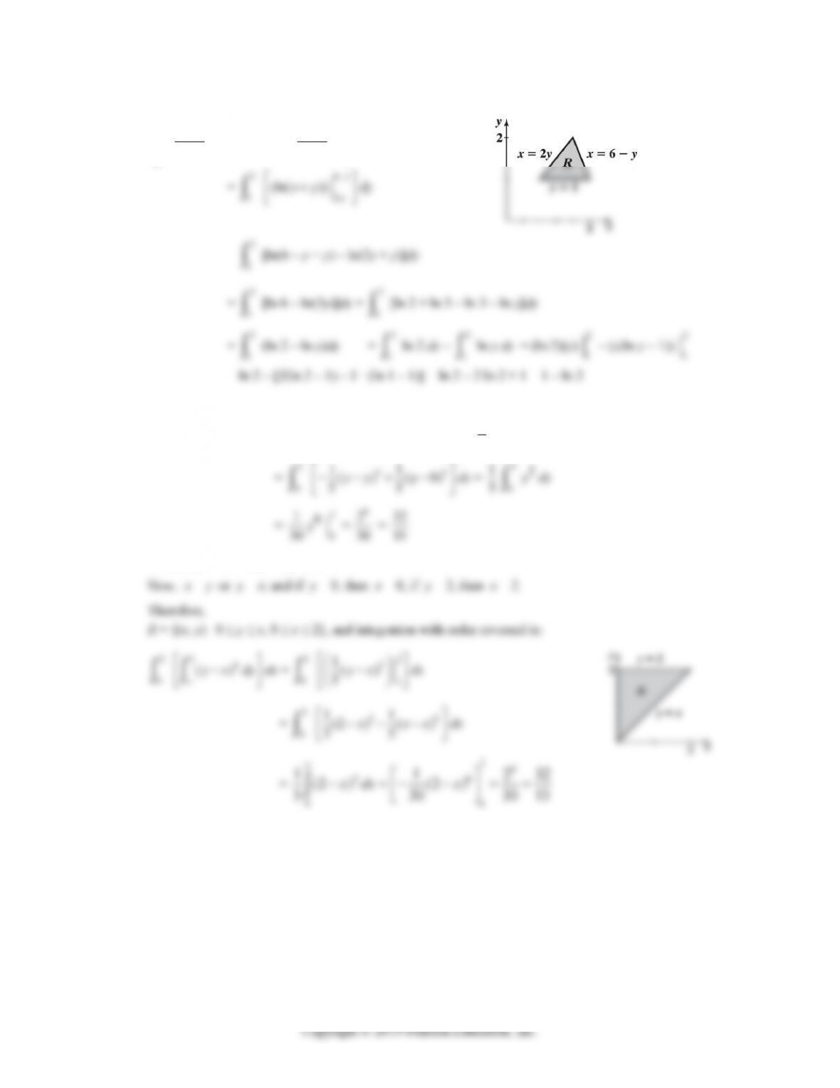
32. R = {(x, y) | 2y ≤ x ≤ 6 – y, 1 ≤ y ≤ 2}
R
1
x
ydA =
2
1
6
2
1
y
y
dx
xy
dy
34.
2
0
0
y
(y – x)4 dx dy =
2
0
4
0
()
y
yxdx
dy =
2
0
5
0
1()
5|y
yx
dy
2
2
R = {(x, y) | 0 ≤ x ≤ y, 0 ≤ y ≤ 2}
x
=
00
(2 ) (2 )
5303015
xdx x
EXERCISE 14-7 14-41
36.
2
0
4
3
x
x
(1 + 2y)dy dx =
2
0
4
3(1 2 )
x
x
ydy
dx
=
2
0
24
3
()
x
x
yy
dx =
2
0
[(4x + 16x2) – (x3 + x6)]dx
2
14-42 CHAPTER 14: MULTIVARIABLE CALCULUS
38.
4
0
2
2
4
y
y
(1 + 2xy)dx dy =
4
0
2
2
4
(1 2 )
y
y
x
ydx
dy
=
4
0
2
2
2
4
()
y
y
xxy
dy
=
4
25
2
(2 4 ) 416
yy
yy
dy
y
y
= 4
6
(4)
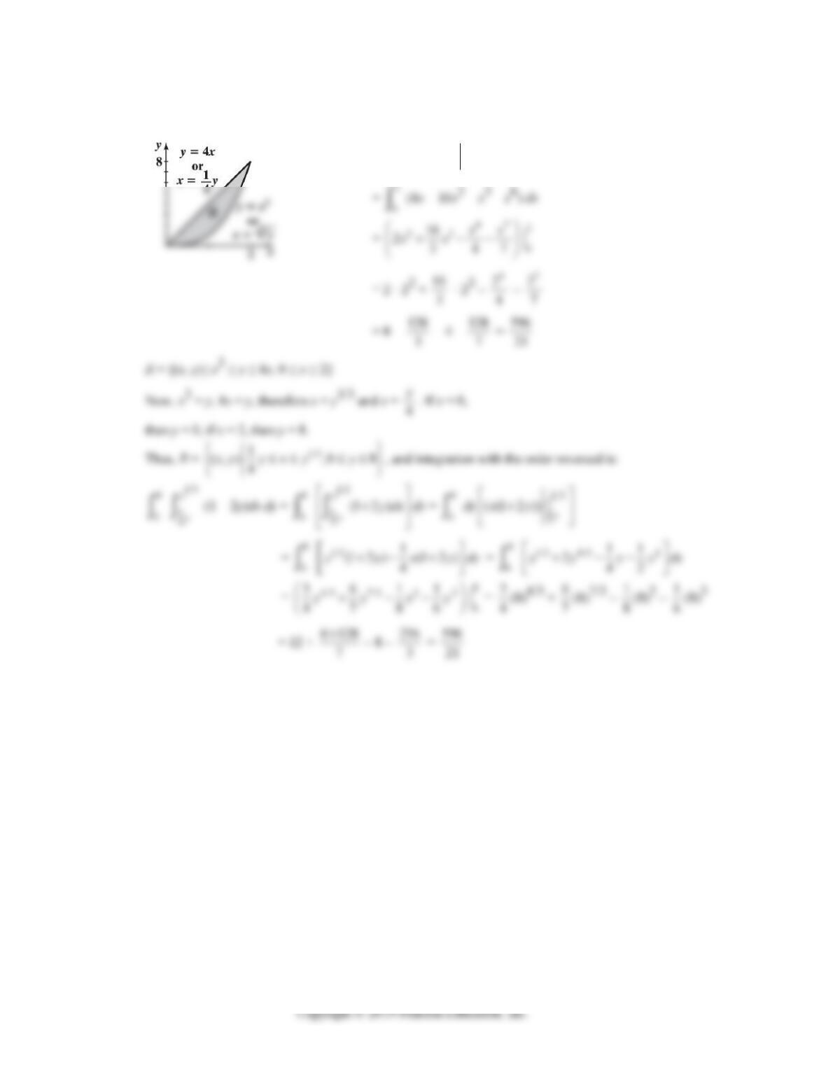
R =
2
(, ) 2 ,0 4
4
y
xy x y y
. Now, x =
2
4
y
or y2 = 4x or
x
2
x
Therefore, R =
2
(, ) 2 ,0 4
4
x
xy y x x
.
4
0
2
2
4
y
y
(1 + 2xy)dx dy =
4
0
2
2
4
x
x
(1 + 2xy)dy dx =
4
0
2
22
4
()
x
x
yxy
dx
25
x
25
x
x
6
4
40. V =
R
(x – y)2 dA
R = {(x, y) | x ≤ y ≤ 2, 0 ≤ x ≤ 2}
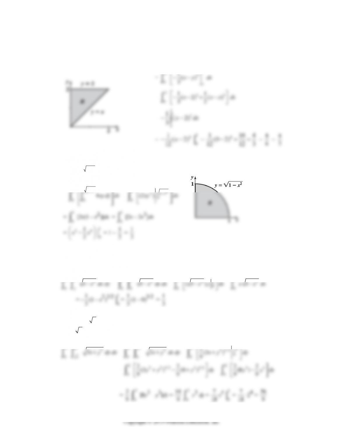
EXERCISE 14-7 14-43
Therefore,
V =
2
0
2
x
(x – y)2 dy dx =
2
0
22
()
x
x
ydy
dx
2
x
42. V =
1
0
1
0
2
x
4xy dy dx
1
1
2
x
1
21
2
44. R = {(x, y) | y ≤ x ≤ 1, 0 ≤ y ≤ 1}
Now, reversing the order will result in
R = {(x, y) | 0 ≤ y ≤ x, 0 ≤ x ≤ 1}. Therefore,
1
x
1
2
1
x
2
1
2
0
x
1
14-44 CHAPTER 14: MULTIVARIABLE CALCULUS
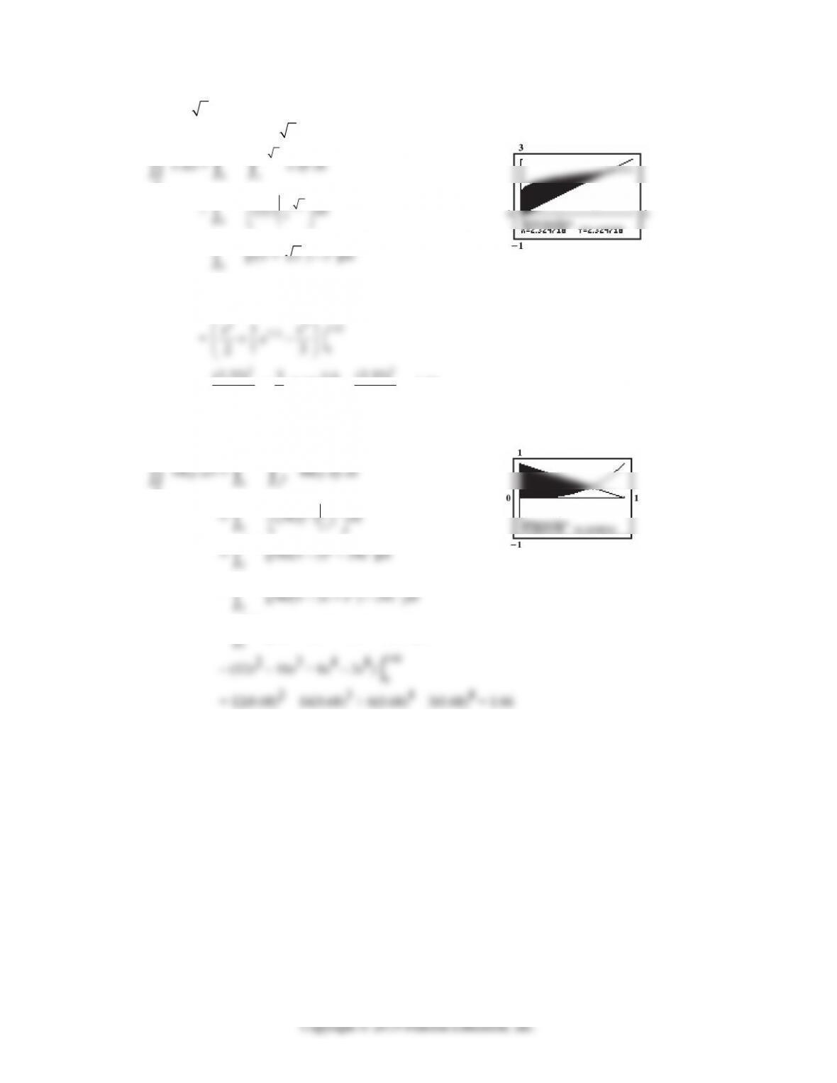
48. y = 1 + 3
x
, y = x, x = 0
R = {(x, y) | x ≤ y ≤ 1 + 3
x
, 0 ≤ x ≤ 2.32}
x
2.32
13
x
=
2.32
0
[x + x4/3 – x2]dx
23
x
=
(2.32)
2 + 3
7(2.32)7/3 –
(2.32)
3 = 1.58
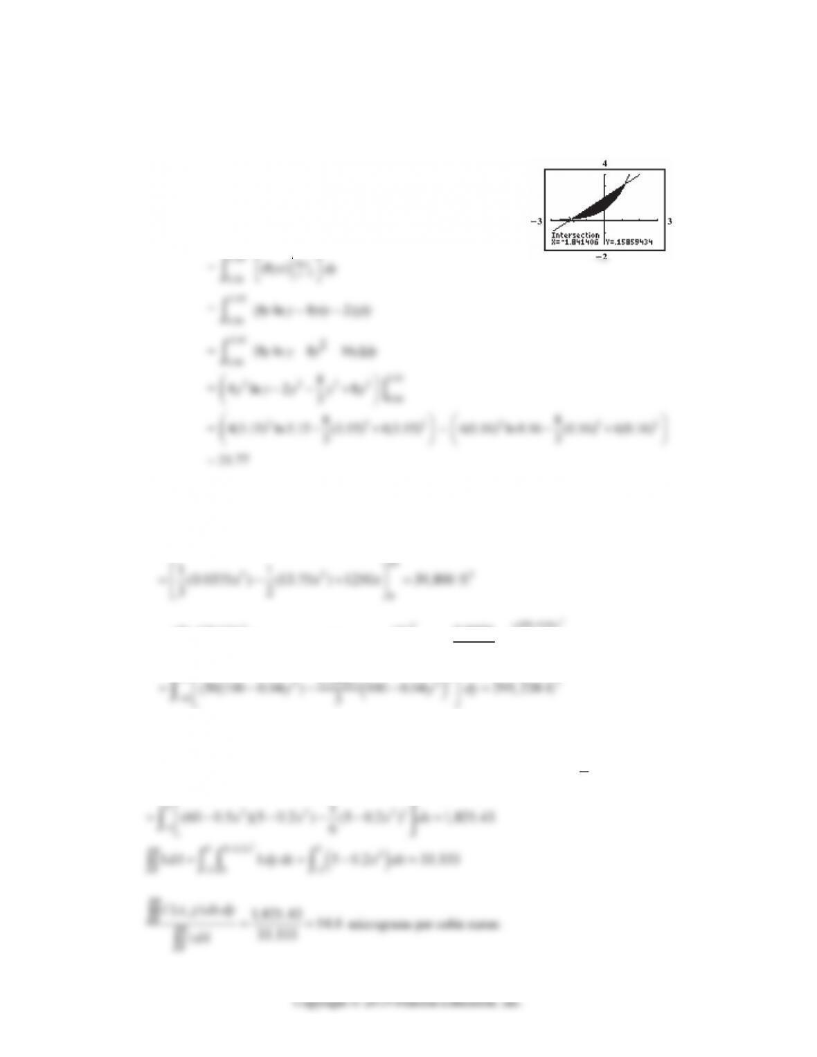
50. y = x3, y = 1 – x, y = 0
R = {(x, y) | x3 ≤ y ≤ 1 – x, 0 ≤ x ≤ 0.68}
x
0.68
1
x
=
0.68
[24x – 48x2 + 24x3 – 24x7]dx
EXERCISE 14-7 14-45
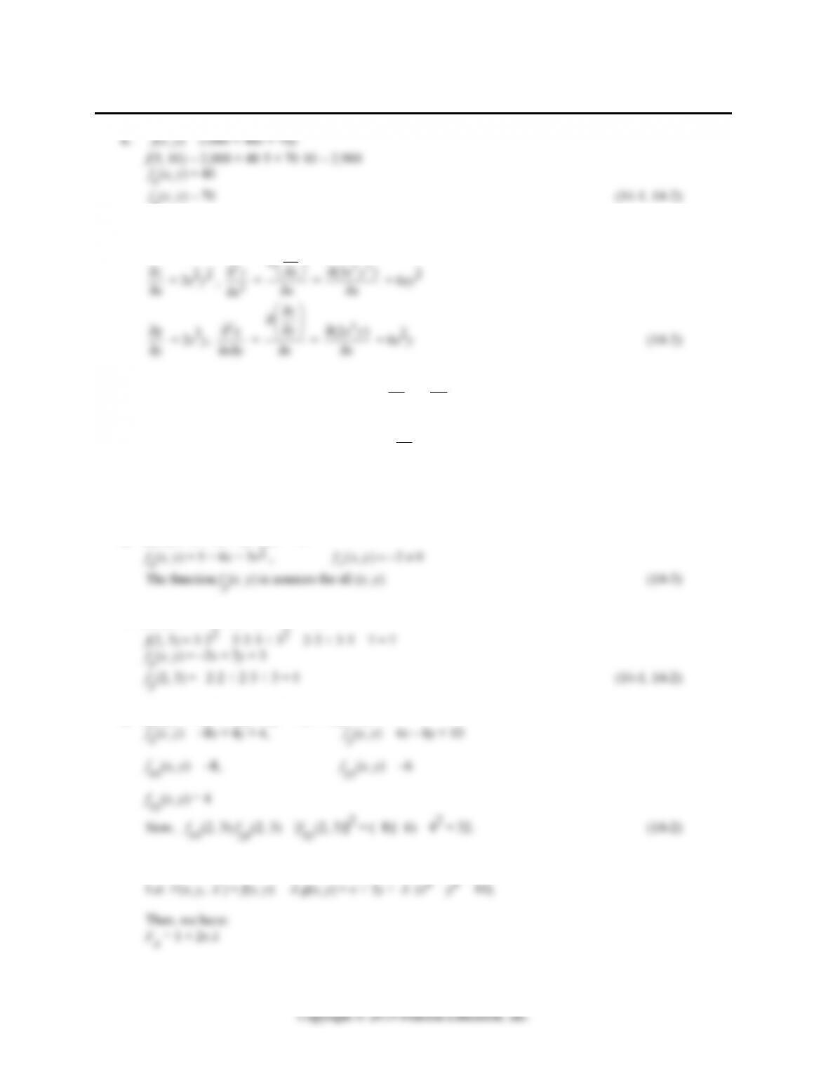
52. y = ex, y = 2 + x
R = {(x, y) | ex ≤ y ≤ 2 + x, –1.84 ≤ x ≤ 1.15} Regular x region
= {(x, y) | y – 2 ≤ x ≤ ln y, 0.16 ≤ y ≤ 3.15} Regular y region
R
8y dA =
1.15
1.84
2
x
e
x
8y dy dx
=
3.15
0.16
ln
2
y
y
8y dx dy
3.15
ln
54.
50 0.3
40 50 0.3 40
00 0 0
40 40 2
00
(25 0.125 ) (25 0.125 )
(25 0.125 )(50 0.3 ) (0.0375 13.75 1250)
x
x
V x dy dx x y dx
x
xdx x x dx
56.
2
2100 0.04
50 100 0.04 50
23
50 0 50 0
0.0025
50 0.0025 50 3
y
y
V x dx dy x x dy
58. 22222
60 0.5 60 0.5( ) 60 0.5 0.5 .Cd xy xy
2
250.2
550.2 5
22 2 3
50 5 0
1
( , ) 60 0.5 0.5 (60 0.5 ) 6
x
x
CxydA x y dydx x y y dx
2
550.2 5 2
x
14-46 CHAPTER 14: MULTIVARIABLE CALCULUS
CHAPTER 14 REVIEW
2. z = x3y2
2
z
22
x
x
x
3.
32
22 32
(6 4) 6 4 6 4 () 2 2 ()
32
yy
x
yydyxydy ydyx CxxyyCx
(14-6)
4.
2
22 2 22
(6 4) 6 4 6 4 () 3 4 ()
2
x
x
y y dx y x dx y dx y yx E y x y xy E y
(14-6)
5.
1
0
1
0
4xy dy dx =
1
0
1
0
4
x
ydy
dx =
1
0
1
11
22
00
0
221xy dx x dx x
(14-6)
6. f(x, y) = 6 + 5x – 2y + 3x2 + x3
7. f(x, y) = 3x2 – 2xy + y2 – 2x + 3y – 7
8. f(x, y) = –4x2 + 4xy – 3y2 + 4x + 10y + 81
9. f(x, y) = x + 3y and g(x, y) = x2 + y2 – 10.
CHAPTER 14 REVIEW 14-47
Fy = 3 + 2y
F
= x2 + y2 – 10
Setting Fx = Fy =
F
= 0, we obtain:
From the first equation, x = – 1
2
; from the second equation, y = – 3
2
.
Substituting these into the third equation gives:
2
1
4
+ 2
9
4
– 10 = 0
10.
k
x
k
y kk
x
y 2
k
x
2
4
12
10
24
40
4
16
1k
xk = 20,
1k
yk = 32,
1k
xkyk = 130,
1k
x2
Substituting these values into the formulas for a and b, we have:
444
4
kk k k
x
yxy
444
14-48 CHAPTER 14: MULTIVARIABLE CALCULUS
Thus, the least squares line is: y = ax + b = –1.5x + 15.5
When x = 10, y = –1.5(10) + 15.5 = 0.5. (14-5)
11.
(4x + 6y) dA =
1
1
2
1
(4x + 6y) d y d x =
1
1
2
1
(4 6 )
x
ydy
dx =
1
1
2
2
1
(4 3 )
x
yy dx
1
1
x
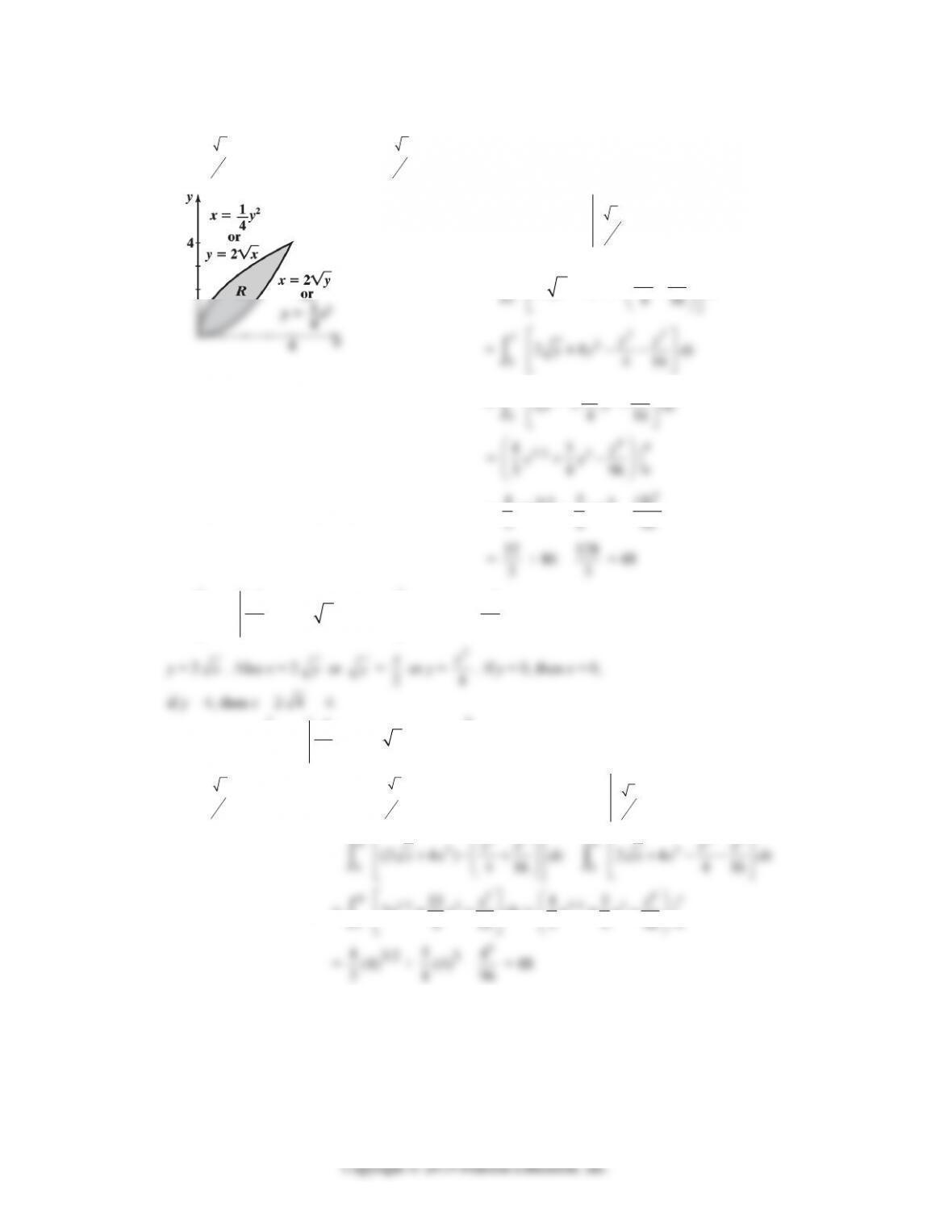
12. R = {(x, y) | y ≤ x ≤ 1, 0 ≤ y ≤ 1}
R is a regular y-region.
(R is also a regular x-region.)
1
1
x
x
R
0
=
1
[(3 + y) – (3y + y3/2)] dy
1
1
13. f(x, y) = ex2+2y
14. f(x, y) = (x2 + y2)5
15. f(x, y) = x3 – 12x + y2 – 6y
1
y
(1,1)
CHAPTER 14 REVIEW 14-49
For the critical point (2, 3):
fxx(2, 3) = 12 > 0
fxy(2, 3) = 0
fyy(2, 3) = 2
16. Step 1: Maximize f(x, y) = xy
Subject to: g(x, y) = 2x + 3y – 24 = 0
Step 2: F(x, y,
) = f(x, y) +
g(x, y) = xy +
(2x + 3y – 24)
Step 3: Fx = y + 2
= 0 (1)
Step 4: Since (6, 4, –2) is the only critical point for F, we conclude that
17. Step 1: Minimize f(x, y, z) = x2 + y2 + z2
Subject to: 2x + y + 2z = 9 or g(x, y, z) = 2x + y + 2z – 9 = 0
14-50 CHAPTER 14: MULTIVARIABLE CALCULUS
Substituting these into (4), we obtain:
Step 4: Since (2, 1, 2, –2) is the only critical point for F, we conclude that
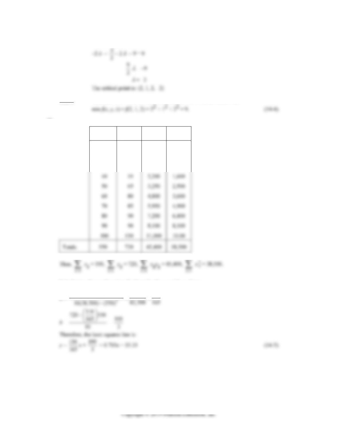
18.
k
x
k
y kk
x
y 2
k
x
10
20
30
50
45
50
500
900
1,500
100
400
900
1k
xk = 550,
1k
yk = 720,
1k
xkyk = 45,400,
1k
x2
Substituting these values into the formulas for a and b, we have:
10(45, 400) (550)(720) 58,000 116
CHAPTER 14 REVIEW 14-51
19. 1
()()badc
R
f(x, y) dA = 1
[8 ( 8)](27 0)
8
8
27
0
x2/3y1/3dy dx
x
8
27 5
8
8
(14-6)
20. V =
R
(3x2 + 3y2) dA =
1
0
1
1
(3x2 + 3y2) dy dx =
1
0
122
1
(3 3 )
x
ydy
dx
x
(14-6)
21. f(x, y) = x + y; –10 ≤ x ≤ 10, –10 ≤ y ≤ 10
Prediction: average value = f(0, 0) = 0.
Verification:
x
10 10
1()
x
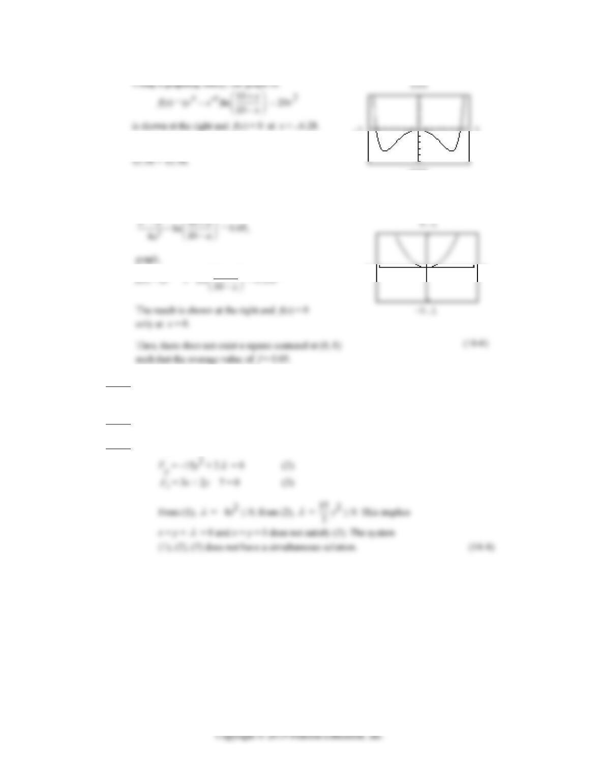
22. f(x, y) = 10
x
e
y
(A) S = {x, y) | –a ≤ x ≤ a, –a ≤ y ≤ a}
The average value of f over S is given by:
1
[()][()] 10
x
aa
aa
edx dy
aaaa y
= 2
1
10
4
a
x
a
aa
edy
y
a
1
aa
a
ee
1
aa
a
ee dy
14-52 CHAPTER 14: MULTIVARIABLE CALCULUS
Copyright © 2019 Pearson Education, Inc.
f(x) = (ex – e-x)ln 10
The dimensions of the square are:
7-7
-500
(B) To determine whether there is a square centered at (0, 0) such that
aa
23. Step 1: Extremize f(x, y) = 4x3 – 5y3
subject to g(x, y) = 3x + 2y – 7 = 0.
Step 2: F(x, y,
) = 4x3 – 5y3 +
(3x + 2y – 7)
Step 3: Fx = 12x2 + 3
= 0 (1)
CHAPTER 14 REVIEW 14-53
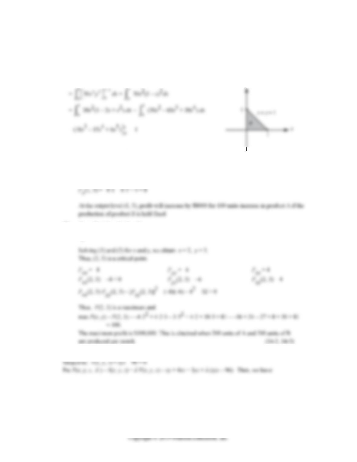
24. R is the region shown in the figure; it is a regular x-region and a regular y-region. F(x, y) = 60x2y ≥ 0 on R
so
V =
R
60x2y dA =
1
0
1
0
x
60x2y dy dx (treating R as an x-region)
11
22
1
(14-7)
25. P(x, y) = –4x2 + 4xy – 3y2 + 4x + 10y + 81
(A) Px(x, y) = –8x + 4y + 4
(B) Px = –8x + 4y + 4 = 0 (1)
Py = 4x – 6y + 10 = 0 (2)
26. Minimize S(x, y, z) = xy + 4xz + 3yz
Subject to: V(x, y, z) = xyz – 96 = 0
Put F(x, y, z,
) = S(x, y, z) +
V(x, y, z) = xy + 4xz + 3yz +
(xyz – 96). Then, we have:
14-54 CHAPTER 14: MULTIVARIABLE CALCULUS
Fx = y + 4z +
yz = 0 (1)
Fy = x + 3z +
xz = 0 (2)
F
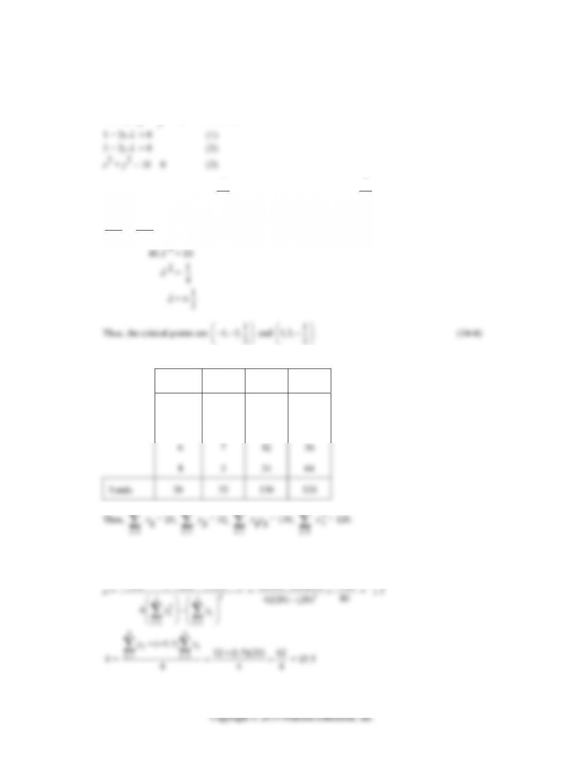
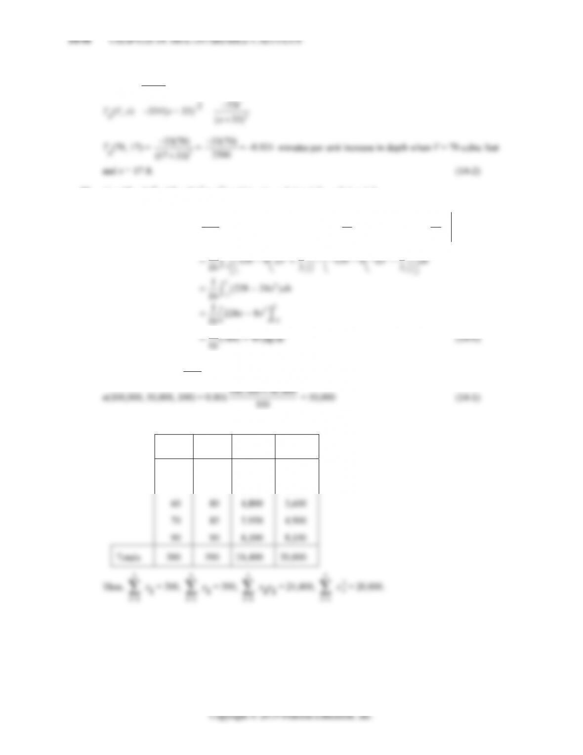
27.
k
x
k
y kk
x
y 2
k
x
1
3
5
2.0
3.1
4.3
2.0
9.3
21.5
1
9
25
Totals 15 16.1 54.6 55
5
5
5
5
a = 2
5(54.6) (15)(16.1) 31.5
28. N(x, y) = 10x0.8y0.2
(A) Nx(x, y) = 8x-0.2y0.2
N
x(40, 50) = 8(40)-0.2(50)0.2 ≈ 8.37
CHAPTER 14 REVIEW 14-55
Copyright © 2019 Pearson Education, Inc.
approximately 8.36 and the marginal productivity of capital is approximately 1.67. Management
should encourage increased use of labor.
(B) Step 1: Maximize the production function N(x, y) = 10x0.8y0.2
Step 2: F(x, y,
) = 10x0.8y0.2 +
(100x + 50y – 10,000)
Step 3: Fx = 8x-0.2y0.2 + 100
= 0 (1)
F
From equation (1),
=
0.2
0.2
0.08y
x
, and from (2),
=
0.8
0.8
0.04
x
.
Thus,
0.2
0.8
Substituting into (3) yields:
200y + 50y = 10,000
(C) Average number of units
=
40
0.8 1.2
100 40 100
0.8 0.2
50 20 50 20
1110
10
(100 50)(40 20) (50)(20) 1.2
xy
x
ydydx dx
1
100
10
1.2 1.2
40 20
100
1.2 1.2
40 20
·
100
1.8
x
Copyright © 2019 Pearson Education, Inc.
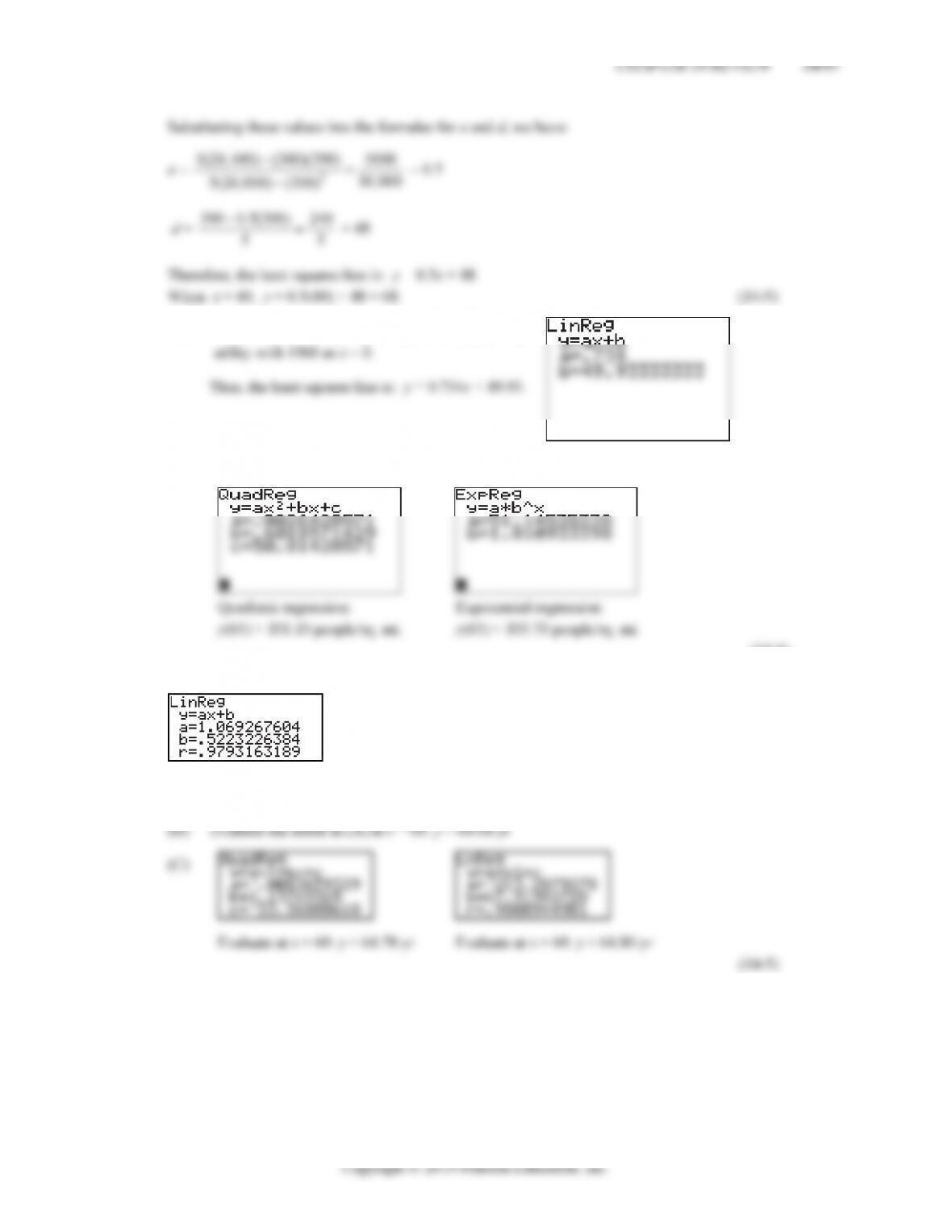
33. (A) We use the linear regression feature on a graphing
(B)The year 2025 corresponds to x = 65; y(65) ≈ 97.64 people/sq. mi.
(C)
(14-5)
34.
(A) The least squares line is y ≈ 1.069x + 0.522.