Inventory Models
Chapter 14
Inventory Models
Learning Objectives
1. Learn where inventory costs occur and why it is important for managers to make good inventory
policy decisions.
2. Learn the economic order quantity (EOQ) model.
7. Know how to make order quantity and reorder point decisions when demand must be described by a
probability distribution.
8. Learn about lead time demand distributions and how they can be used to meet acceptable service
levels.
9. Be able to develop order quantity decisions for periodic review inventory systems.
10. Understand the following terms:
inventory holding costs backorder
cost of capital quantity discounts
ordering costs goodwill costs
Chapter 14
14 –
2
Solutions:
1. a.
*22(3600)(20) 438.18
0.25(3)
o
h
DC
QC
= = =
b.
3600 (5) 72
250
r dm= = =
2. Annual Holding Cost
11
(438.18)(0.25)(3) $164.32
22
h
QC ==
3.
*22(5000)(32) 400
2
O
h
DC
QC
= = =
5000 20 units per day
250 250
D
d= = =
a. r = dm = 20(5) = 100
Since r Q*, both inventory position and inventory on hand equal 100.
b. r = dm = 20(15) = 300
Since r Q*, both inventory position and inventory on hand equal 300.
14 –
3
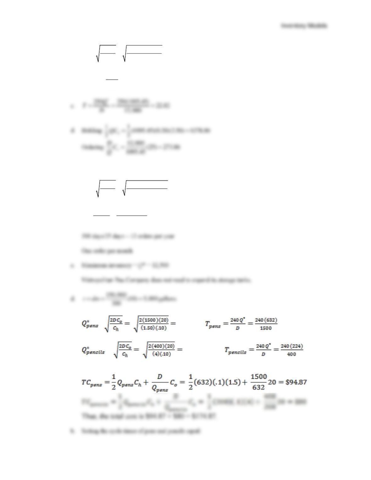
4. a.
*22(12,000)(25) 1095.45
(0.20)(2.50)
o
h
DC
QC
= = =
b.
1200 (5) 240
250
r dm= = =
Total Cost = $547.72
5. a.
*22(150,000)(250) 12,500
0.48
o
h
DC
QC
= = =
b.
*
300 300(12,500) 25
150,000
Q
TD
= = =
days
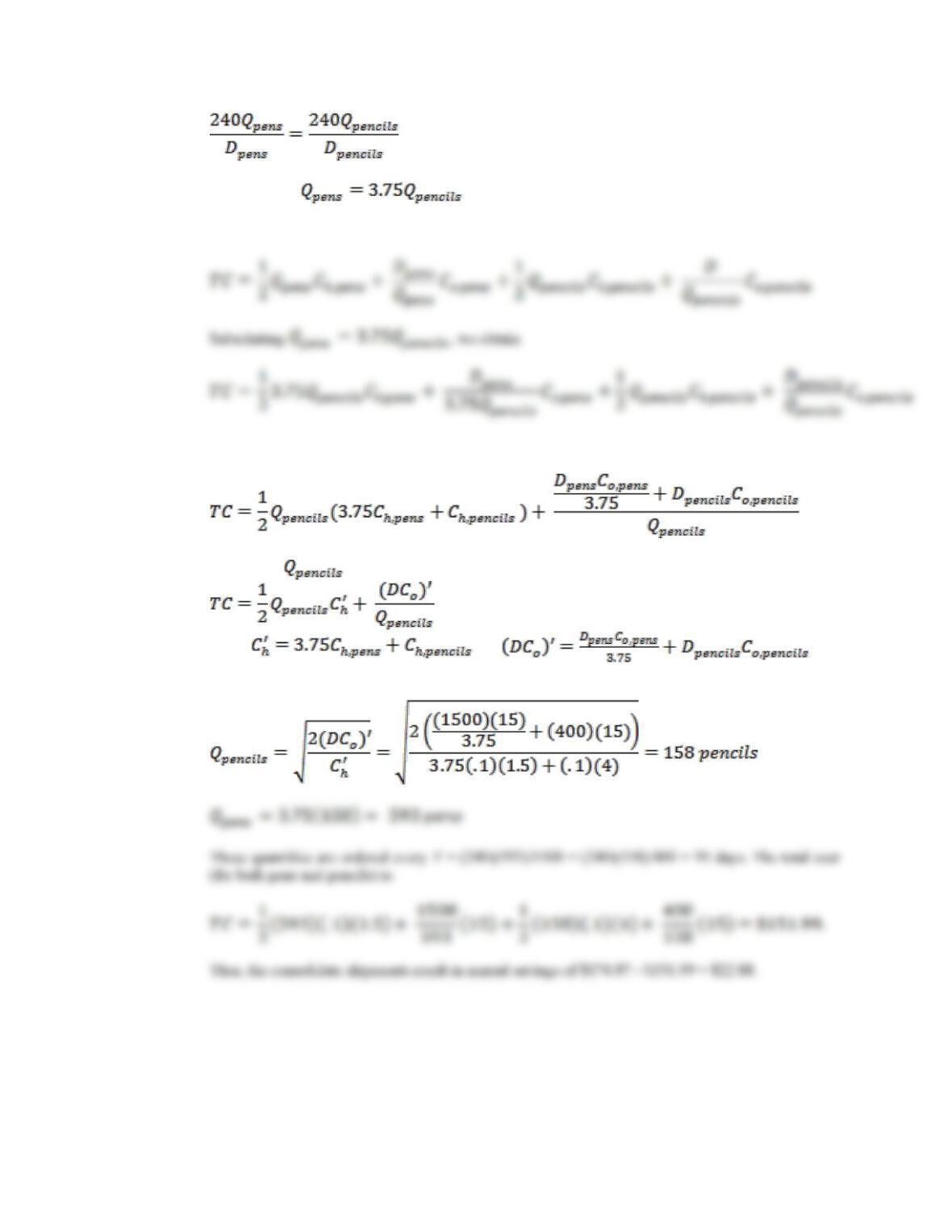
6. a. = 632 pens, = 101 days
= 200 pencils, = 120
days
Chapter 14
14 –
4
which implies .
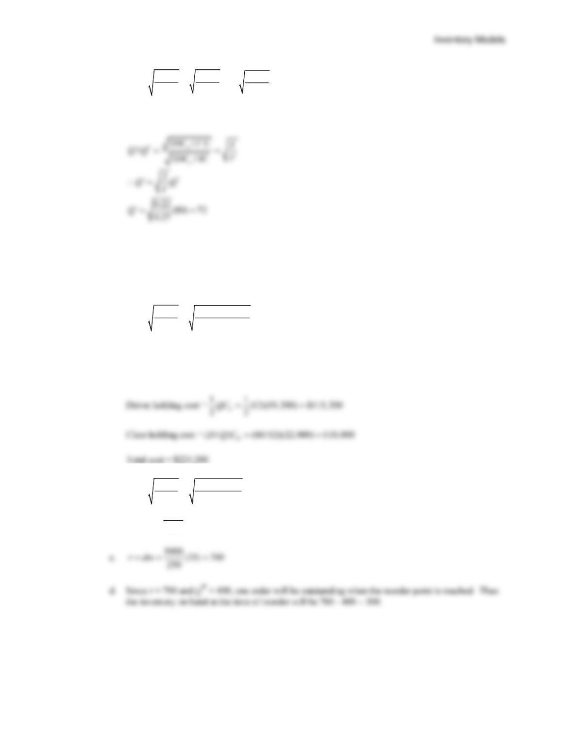
The total cost (for both pens and pencils) is:
Combining like terms:
Solving for by observing that this total cost equation is the same as
where and .
Thus,
14 –
5
7.
*22
oo
h
DC DC
QC IC
==
2
‘‘
o
DC
QIC
Where
‘Q
is the revised order quantity for the new carrying charge
‘I
. Thus
8. Annual Demand D = (5/month)(12 months) = 60
Ordering Cost = Fixed Cost per class = $22,000
Holding Cost = ($1,600/month)(12 months) = $19,200 per year for one driver
*22(60)(22,000) 11.73
(19,200)
o
h
DC
QC
= = =
Use 12 as the class size.
D/Q* = 60/12 = 5 classes per year
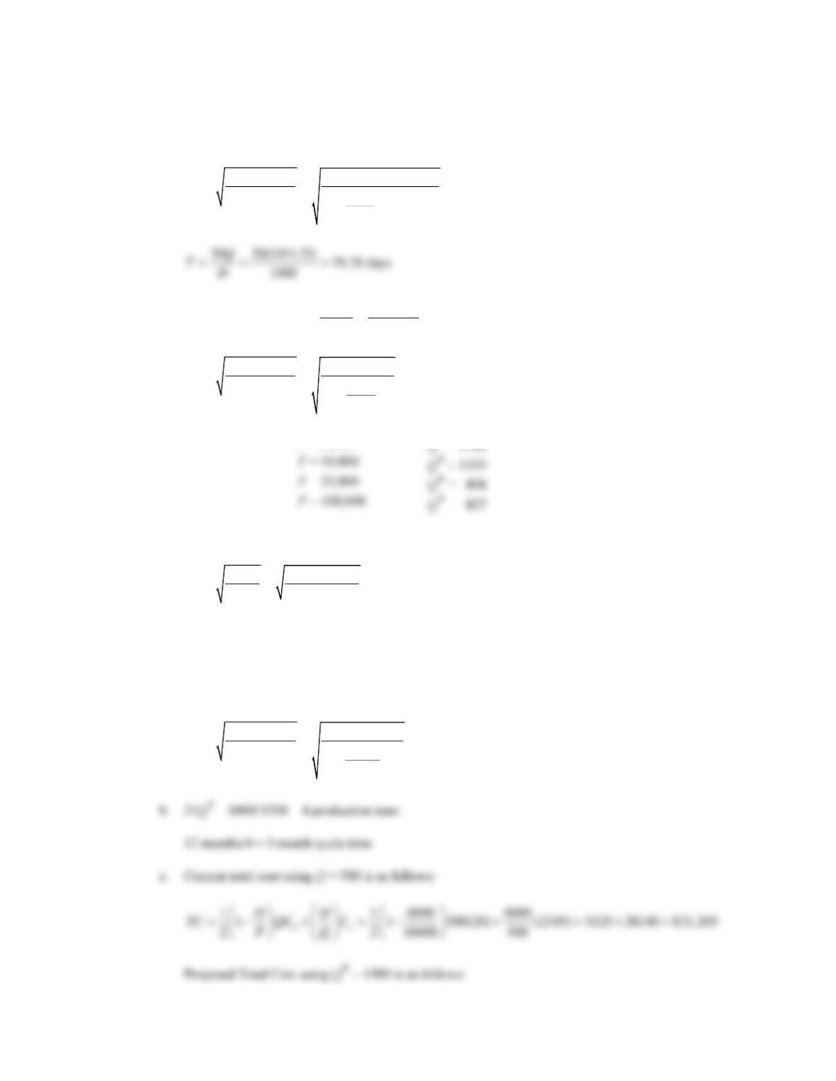
9. a.
*22(5000)(80) 400
(0.25)(20)
o
h
DC
QC
= = =
b.
5000 (12) 240
250
r dm= = =
Chapter 14
14 –
6
10. This is a production lot size model. However, the operation is only six months rather than a full
year. The basis for analysis may be for periods of one month, 6 months, or a full year. The
inventory policy will be the same. In the following analysis we use a monthly basis.
22(1000)(150)
* 1414.21
1000
(1 / ) 1 (0.02)(10)
4000
o
h
DC
QD P C
= = =
−
−
Production run length =
1414.21 7.07
/ 20 4000/ 20
Q
P==
days
11.
22(6400)(100)
*6400
(1 / ) 12
o
h
DC
QD P C
P
==
−
−
EOQ Model:
22(6400)(100)
* 800
2
o
h
DC
QC
= = =
Production Lot Size Q* is always greater than the EOQ Q* with the same D, C0, and Ch values.
As the production rate P increases, the recommended Q* decreases, but always remains greater than
the EOQ Q*.
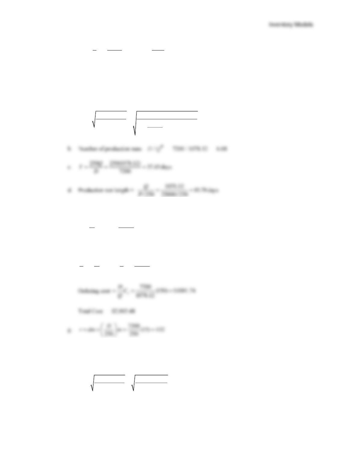
12. a.
22(6000)(2345)
* 1500
6000
(1 / ) 1 20
16000
o
h
DC
QD P C
= = =
−
−
14 –
7
1 6000 6000
1 1500(20) (2345) 9375 9380 $18,755
2 16000 1500
TC
= − + = + =
Change to Q* = 1500
Savings = $31,265 – $18,755 = $12,510
12,510/31,265 = 40% savings over current policy
13. a.
22(7200)(150)
* 1078.12
7200
(1 / ) 1 (0.18)(14.50)
25000
o
h
DC
QD P C
= = =
−
−
e. Maximum Inventory
7200
1 1 (1078.12) 767.62
25000
DQ
P
− = − =
f. Holding Cost
1 1 7200
1 1 (1078.12)(0.18)(14.50) $1001.74
2 2 25000
h
DQC
P
− = − =
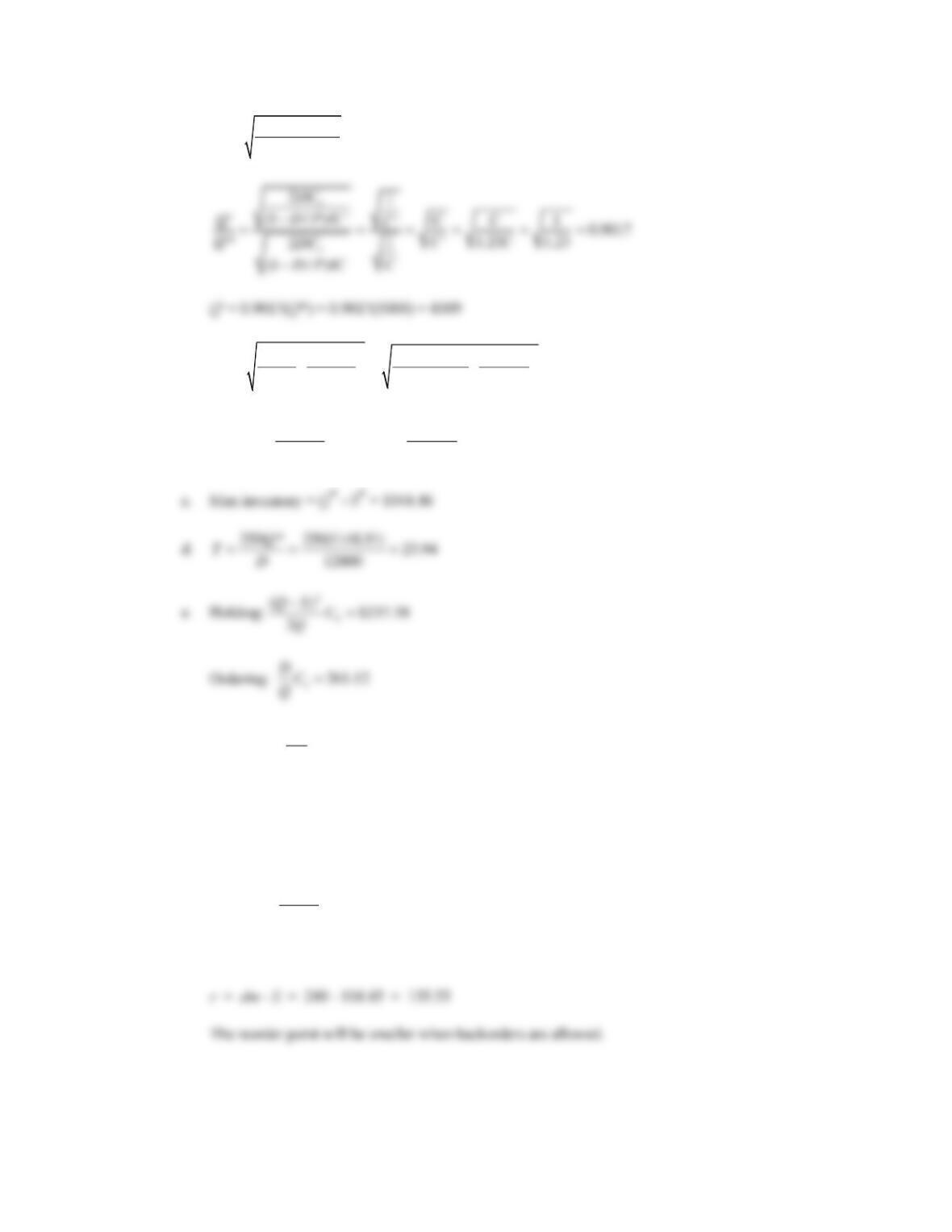
14. C = current cost per unit
C ‘ = 1.23 C new cost per unit
Let Q‘ = new optimal production lot size
*0
22
5000
(1 / ) (1 / )
o
h
DC DC
QD P C D P IC
= = =
−−
Chapter 14
14 –
8
2
‘(1 / ) ‘
o
DC
QD P IC
=−
15. a.
22(1200)(25) 0.50 5
* 1148.91
0.50 0.50
o h b
hb
DC C C
QCC
++
= = =
b.
0.50
* * 1148.91 104.45
0.50 5
h
hb
C
SQ
CC
= = =
++
Backorder:
223.74
2b
SC
Q=
Total Cost: $522.24
The total cost for the EOQ model in problem 4 was $547.72. Allowing backorders reduces the total
cost.
16.
12000 5 240
250
r dm
= = =
With backorder allowed the reorder point should be revised to
14 –
9
17. EOQ Model
22(800)(150)
* 282.84
3
o
h
DC
QC
= = =
Total Cost
0
1 282.84 800
3 (150) $848.53
2 2 282.84
h
D
QC C
Q
= + = + =
Total Cost
22
() 344.02 395.63 51.60 $791.25
22
h o b
Q S D S
C C C
Q Q Q
−
= + + = + + =
Cost Reduction with Backorders allowed
$848.53 – 791.25 = $57.28 (6.75%)
Both constraints are satisfied:
18. Reorder points:
EOQ Model:
800 20 64
250
r dm
= = =
Backorder Model: r = dm – S = 24.44
Chapter 14
14 –
10
b.
22(480)(15) 0.20(60) 45
* 39
(0.20)(60) 45
o h b
hb
DC C C
QCC
++
= = =
c. Length of backorder period
8.21 5.13
480/300
S
d
= = =
days
d. Backorder case since the maximum wait is only 5.13 days and the cost savings is
$415.70 – 369.36 = $46.34 (11.1%)
20.
2o
h
DC
QC
=
11
2(120)(20) 25.30 25
0.25(30)
QQ= = =
Category
Unit Cost
Order
Quantity
Holding
Cost
Order Cost
Purchase
Cost
Total
Cost
1
30.00
25
93.75
96
3600
$3,789.75
2
28.50
50
178.13
48
3420
$3,646.13
3
27.00
100
337.50
24
3240
$3,601.50
14 –
11
21.
2o
h
DC
QC
=
Since Q1 is over its limit of 99 units, Q1 cannot be optimal (see problem 23). Use Q2 = 143.59 as
the optimal order quantity.
Total Cost:
1139.28 139.28 4,850.00 $5,128.56
2ho
D
QC C DC
Q
= + + = + + =
22. D = 4(500) = 2,000 per year
Co = $30
I = 0.20
C = $28
Annual cost of current policy: (Q = 500 and C = $28)
TC = 1/2(Q)(Ch) + (D/Q)Co + DC
= 1/2(500)(0.2)(28) + (2000/500)(30) + 2000(28)
= 1400 + 120 + 56,000 = 57,520
Order Quantity
Ch
Q*
Q to obtain
Discount
TC
0-99
(0.20)(36) = 7.20
129
*
—
100-199
(0.20)(32) = 6.40
137
137
64,876
200-299
(0.20)(30) = 6.00
141
200
60,900
300 or more
(0.20)(28) = 5.60
146
300
57,040
*Cannot be optimal since Q* > 99.
Chapter 14
14 –
12
23.
1
2o
D
TC QIC C DC
Q
= + +
At a specific Q (and given I, D, and C0), since C of category 2 is less than C of category 1, the TC
for 2 is less than TC for 1.
catego ry 1
catego ry 2
TC
Thus, if the minimum cost solution for category 2 is feasible, there is no need to search category 1.
From the graph we can see that all TC values of category 1 exceed the minimum cost solution of
category 2.
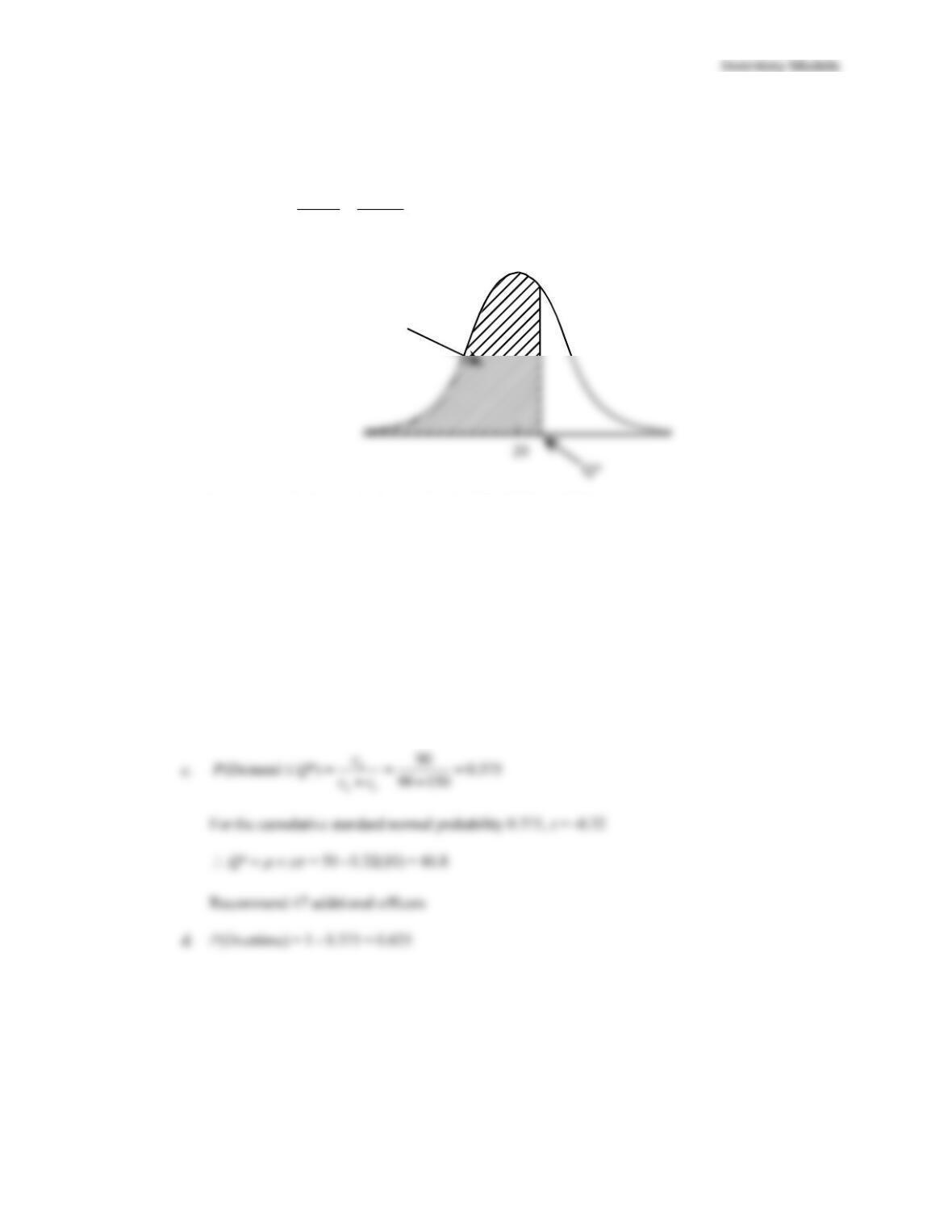
24. a. Cost of overestimation, co = $9
Cost of underestimation, cu = $10 – $9 -$0.50 = $0.50
b. Cost of overestimation, co = $9 – $8 = $1
Cost of underestimation, cu = $10 – $9 -$0.50 = $0.50
P( demand ≤ Q*) =
14 –
13
25. a. co = 80 – 50 = 30
cu = 125 – 80 = 45
45
( *) 0.60
45 30
u
uo
c
P D Q cc
= = =
++
For the cumulative standard normal probability 0.60, z = 0.25
Q* = 20 + 0.25(8) = 22
b. P(Sell All) = P(D Q*) = 1 – 0.60 = 0.40
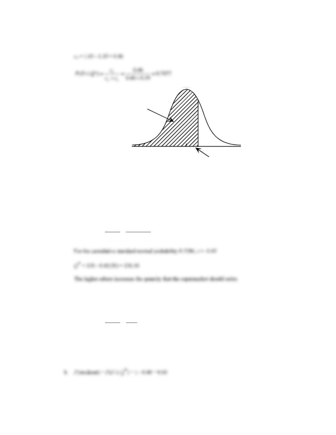
26. a. co = $150
b. The city would have liked to have planned for more additional officers at the $150 per officer rate.
However, overtime at $240 per officer will have to be used.
cu = $240 – $150 = $90
= 8
P(D Q*) = 0.60
Chapter 14
14 –
14
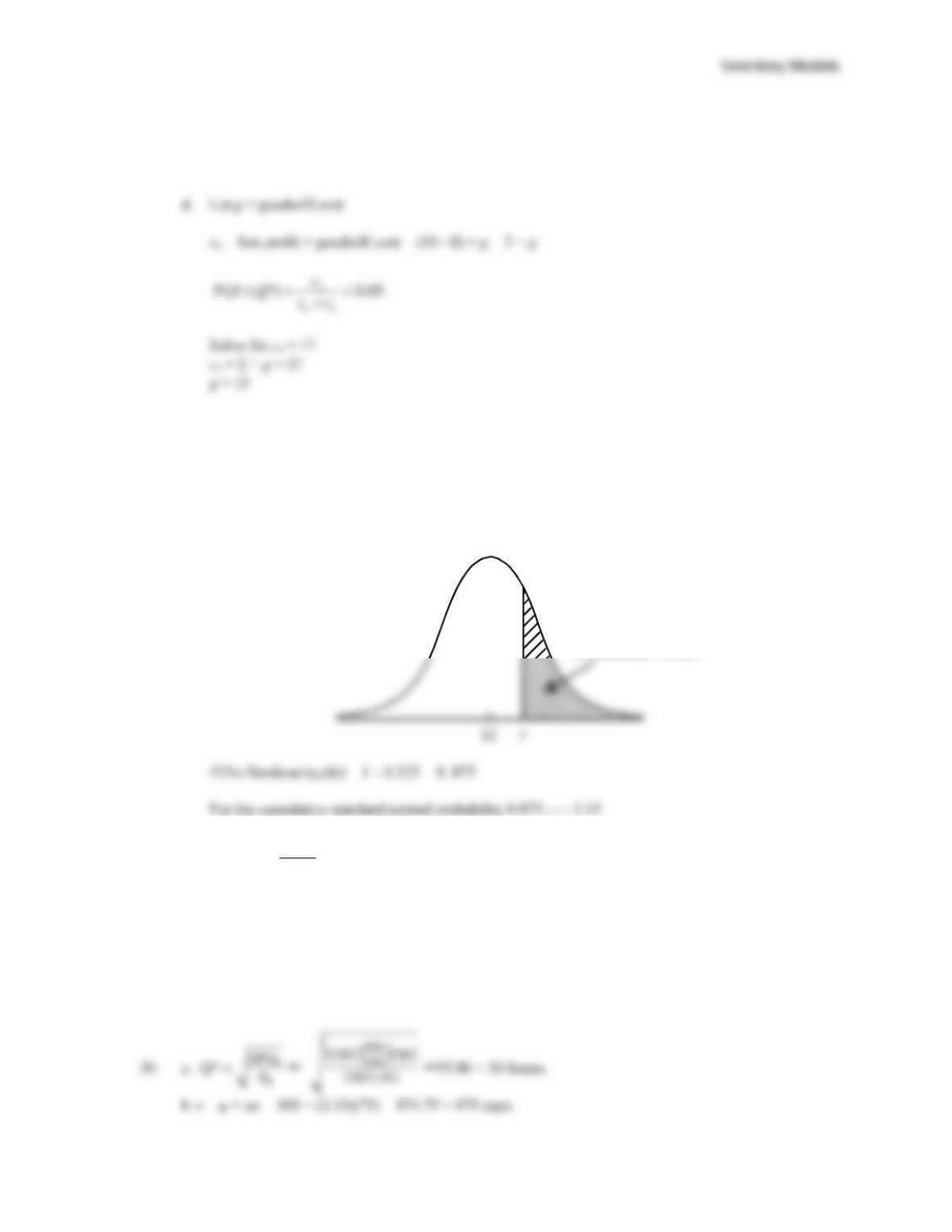
27. a. co = 1.19 – 1.00 = 0.19
For the cumulative standard normal probability 0.7077, z = 0.55
Q* = 150 + 0.55(30) = 166.5
b. P(Stockout) = P(D Q*) = 1 – 0.7077 = 0.2923
c. co = 1.19 – 0.25 = 0.94
0.46
( *) 0.3286
0.46 0.94
u
c
P D Q cc
= = =
++
28. a. co = 8 – 5 = 3
cu = 10 – 8 = 2
2
( *) 0.40
23
u
uo
c
P D Q cc
= = =
++
Q* is 40% of way between 700 and 800
Q* = 200 + 0.40(600) = 440
150
= 30
P(D Q*) = 0.7077
Q*
14 –
15
c. P(D Q*) = 0.85 P(Stockout) = 0.15
Q* = 200 + 0.85(600) = 710
29. a. r = dm = (200/250)15 = 12
b. D / Q = 200 / 25 = 8 orders / year
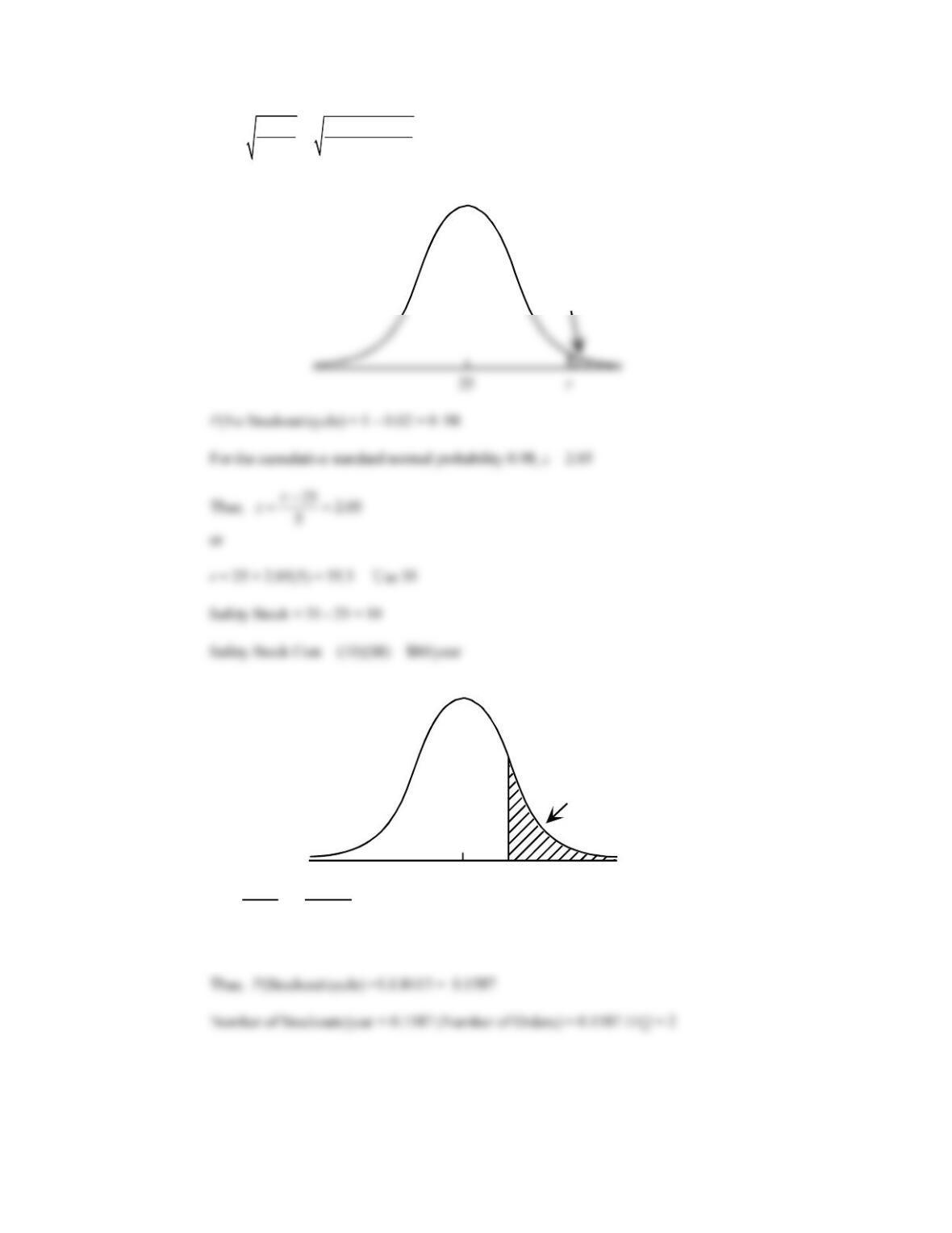
The limit of 1 stockout per year means that
P(Stockout/cycle) = 1/8 = 0.125
Thus,
12 0.15
2.5
r
z−
==
or
r = 12 + 1.15(2.5) = 14.875 Use 15
c. Safety Stock = 3 units
Added Cost = 3($5) = $15/year
= 2.5
Chapter 14
14 –
16
31. a.
22(1000)(25.5)
* 79.84
8
o
h
DC
QC
= = =
b.
c.
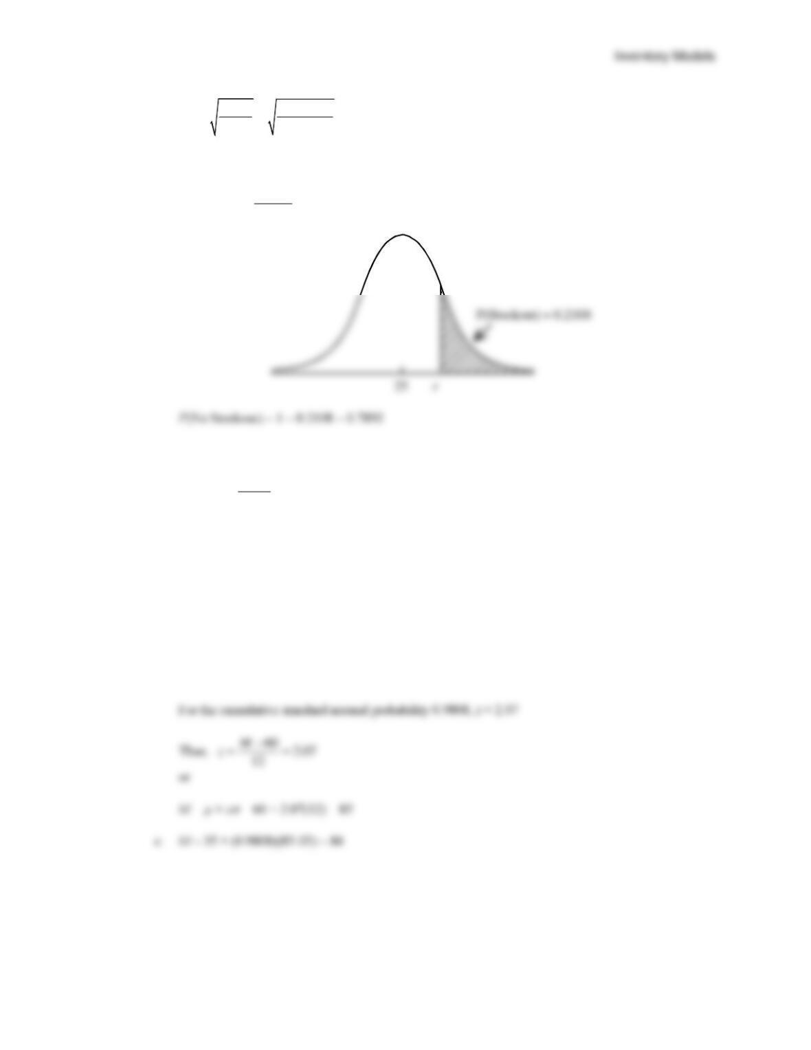
z = r – 25
5 = 30 – 25
5 = 1
The cumulative standard normal probability for z = 1 is 0.8413.
= 5
P(Stockout) = 0.02
25
= 5
P(Stockout) = ?
30
14 –
17
32. a.
22(300)(5)
* 31.62
(0.15)(20)
o
h
DC
QC
= = =
b. D / Q* = 9.49 orders per year
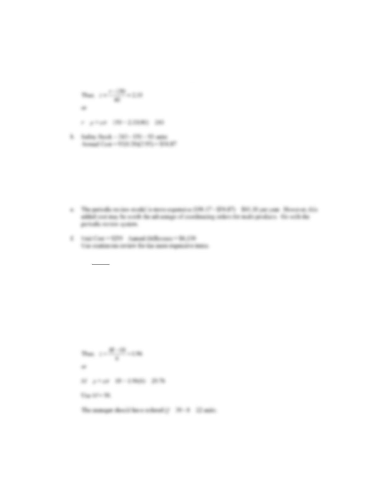
For the cumulative standard normal probability 0.7892, z = 0.80
Thus,
25 0.80
6
r
z−
==
or
r = 15 + 0.80(6) = 19.8 Use 20
c. Safety Stock = 20 – 15 = 5
Safety Stock Cost =5(0.15)(20) = $15
33. a. 1/52 = 0.0192
b. P(No Stockout) = 1 – 0.0192 = 0.9808
PD Q
( ) / * .Stockout = =
202108
= 6
Chapter 14
14 –
18
34. a. P(Stockout) = 0.01 z = 2.33
P(No Stockout) = 1 – 0.01 = 0.99
For the cumulative standard normal probability 0.99, z = 2.33
c. z = 2.33
M = µ + z
= 450 + 2.33(70) = 613 units
d. Safety Stock = 613 – 450 = 163 units
Annual Cost = 163(0.20)(2.95) = $96.17
35. a.
24 18 1.0
6
z−
==
The cumulative standard normal probability for z = 1.0 is 0.8413.
P(Stockout) = 1.0000 – 0.8413 = 0.1587
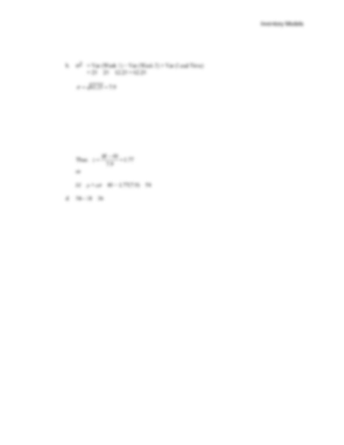
b. P(Stockout) = 0.025
P(No Stockout) = 1 – 0.025 = 0.975
For the cumulative standard normal probability 0.975, z = 1.96
14 –
19
36. a. µ = Week 1 demand + Week 2 demand + Lead Time demand
= 16 + 16 + 8 = 40
c. 26 orders per year
P(Stockout) = 1/26 = 0.0385 per replenishment
P(No Stockout) = 1 – 0.0385 = 0.9615
For the cumulative standard normal probability 0.9615, z = 1.77