EXERCISE 14-4 14-21
Copyright © 2019 Pearson Education, Inc.
28. The constraint g(x, y) = 4x – y + 3 = 0 implies y = 4x + 3. Substituting for y in the function f, the problem
30. Minimize f(x, y) = x2 + 2y2
Critical values: x = 0, 1 – 2e-x2 = 0
x = 0, x = ± ln 2 = ±0.833
2
-2
From the constraint equation, y = 1
2 when x = ±0.833.
(B) F(x, y,
) = x2 + 2y2 +
(yex2 – 1)
Fx = 2x + 2
xyex2 = 0 (1)
14-22 CHAPTER 14: MULTIVARIABLE CALCULUS
Now, y = 1 when x = 0, and y = 1
2 when x = ± ln 2 = ±0.833.
32. Step 1. Maximize production function N(x, y) = 4xy – 8x
Step 2. F(x, y,
) = 4xy – 8x +
(x + y – 60)
Step 3. Fx = 4y – 8 +
= 0 (1)
Fy = 4x +
= 0 (2)
Step 4. Since (29, 31, –116) is the only critical point for F, we conclude that:
34. (A) Step 1. Maximize the production function N(x, y) = 10x0.6y0.4
Step 2. F(x, y,
) = 10x0.6y0.4 +
(30x + 60y – 300,000)
Step 3. Fx = 6x-0.4y0.4 + 30
= 0 (1)
EXERCISE 14-4 14-23
Substituting into (3), we have:
30(3y) + 60y – 300,000 = 0
36. Let x = length, y = width, and z = height.
Step 1. Maximize volume V = xyz
Step 2. F(x, y, z,
) = xyz +
(x + 2y + 2z – 120)
Step 3. Fx = yz +
= 0 (1)
Fy = xz + 2
= 0 (2)
Step 4. Since (40, 20, 20, –400) is the only critical point for F:
max V(x, y, z) = V(40, 20, 20) = 16,000 cubic inches.
38. Step 1. Minimize C(x, y) = x + 2y
Step 2. F(x, y,
) = x + 2y +
(200xy – 25,600)
Step 3. Fx = 1 + 200
y = 0 (1)
Fy = 2 + 200
x = 0 (2)
14-24 CHAPTER 14: MULTIVARIABLE CALCULUS
or
= ± 1
1,600
Step 4. Since 1
16,8, 1, 60 0
is the only critical point for F, min C(x, y) = C(16, 8) = 32.
EXERCISE 14-5
2.
5
45791338
y
5
2 22222
01234 30
x
2
5
22
8. xk y
k x
kyk 2
k
x
1
–2
–2
1
Totals 10 5 25 30
1k
1k
1k
1k
Substituting these values into formulas for slope and y intercept respectively,
we have:
a = 111
nn
kk k k
kkk
n
nxy x y
= 2
4(25) (10)(5)
EXERCISE 14-5 14-27
20. xk y
k x
kyk 2
k
x
0
2
4
–15
–9
–7
0
–18
–28
0
4
16
22. Minimize
F(a, b, c) = (a – b + c + 2)2 + (c – 1)2 + (a + b + c – 2)2 + (4a + 2b + c)2
Fa = 2(a – b + c + 2) + 2(a + b + c – 2) + 8(4a + 2b + c)
Fb = –2(a – b + c + 2) + 2(a + b + c – 2) + 4(4a + 2b + c)
EXERCISE 14-5 14-29
32.
34.
(A) x
k y
k x
kyk 2
k
x
4.5
5.5
3.5
1.5
15.75
8.25
20.25
30.25
1k
1k
1k
1k
Substituting these values in the formulas for a and b, we have:
a = 2
5(58.50) (25)(12.6)
5(127.50) (25)
= –1.80 and b = 12.6 1.80(25)
5
= 11.52
Thus, the least squares line is y = –1.80x + 11.52 which is the demand equation.
(B) Let C(y) be the cost for purchasing y cans. Then
x = 4.70
$4.70.
36.
(A) hk d
k h
kdk 2
k
h
0
1
2
0
7
18
0
7
36
0
1
4
1k
1k
1k
1k
Substituting these values into formulas for a and b, we have:
a = 2
5(259) (10)(86)
5(30) (10)
= 8.7, b = 86 8.7(10)
5
= –0.2
14-30 CHAPTER 14: MULTIVARIABLE CALCULUS
Copyright © 2019 Pearson Education, Inc.
The least squares line for the data is d = 8.7h – 0.2.
Note: d = 8h appears to be approximately correct.
(B) For h = 3.5, d = 8.7(3.5) – 0.2 ≈ 30 days.
38.
EXERCISE 14-6
11
2
xx
6. ln 1 ln 1
(Let ln . Then )
xx
dx dx u x du dx
xx x
11 1
22
8. (A)
12x2y3dx = 12y3
x2 dx (y is treated as a constant.)
x
+ E(y) (The “constant” of integration
(B)
1
12x2y3 dx = 4y3(x3)2
1
|
10. (A)
(4x + 6y + 5) dy =
(4x + 5)dy +
6y dy = (4x + 5)y + 3y2 + C(x)
1
1
1
12. (A) 2
x
yx
dy = x
(y + x2)-1/2 dy
EXERCISE 14-6 14-31
Copyright © 2019 Pearson Education, Inc.
5
x
yxdy = 2x
2
22
14. (A)
ln
x
x
ydx = 1
y
ln
x
x
dx
Let u = ln x, then du = 1
x
dx, and
x
y
x
y
x
y
y
x
ln
x
ln
x
2
u + E(y)
(B)
1
x
ydx = 1
2
y
(ln x)2 1
|e = 1
2
y
[(ln e)2 – (ln 1)2]= 1
2
y
16. (A) 33
22 23
33 3
xy x y x y
ye dy yee dy e ye dy
0
18.
1
0
2
1
12x2y3dx dy =
1
0
223
1
12
x
ydx
dy =
1
0
36y3 dy (see Problem 8)
0
20.
3
4
(4x + 6y + 5)dy dx =
3
4
(4 6 5)
x
ydy
dx
3
2
22.
2
0
5
1
2
x
yxdy dx =
2
0
5
2
1
xdy
yx
dx
x
2
22
y
x
14-32 CHAPTER 14: MULTIVARIABLE CALCULUS
To compute
2
0
2x2
5
x
dx we make the substitution
u = 5 + x2, du = 2x dx:
2x2
5
x
dx =
u1/2 du =
3/2
32
u + C =
3/2
2
3
u + C = 2
3(5 + x2)3/2 + C
x
2
x
= 56 20 5
3
24.
1
2
e
1
e
ln
x
x
ydx dy =
1
2
e
1
ln
exdx
xy
dy
2
26. 33
12 1 2 1
22 8
00 0 0 0
3 3 e ( –1) (from Problem 16)
xy xy x
y e dy y e dy dx e dx
28.
R
x
ydA =
4
1
9
1
x
ydy dx =
4
1
x
3/2
32
y
9
1
|dx =
4
1
x
2
3(93/2 – 1) dx
R
x
y dA =
9
1
4
1
x
ydx dy =
9
1
y
3/2
32
x
4
1
|dy =
9
1
y 2
3(43/2 – 1) dy
2
9
9
EXERCISE 14-6 14-33
30.
R
xey dA =
3
2
2
0
xey dy dx =
3
2
(xey)0
2dx =
3
2
x(e2 – 1)dx = (e2 – 1)
3
2
x dx
2
x
3
21
e(9 – 4) = 5
x
32. Average value = 1
[2 ( 1)](4 1) R
(x2 + y2)dA
34. Average value = 1
[1 ( 1)](2 0) R
x2y3 dA = 1
4
1
1
2
0
x2y3 dy dx
1
y
2dx = 1
1
1
1
36. V =
R
(5 – x)dA =
5
0
5
0
(5 – x)dy dx
5
5dx =
5
1(5 )
5 = 5 25
38. V =
R
e-x-y dA =
1
0
1
0
e-x-y dy dx =
1
0
1
0
e-xe-y dy dx =
1
0
e-x(–e–y)0
1 dx =
1
0
e-x(–e–1 + 1)dx
1
1 = (1 – e-1)2 cubic units
40.
R
xyex2y dA =
2
1
1
0
2
xy
x
ye dx
dy
14-34 CHAPTER 14: MULTIVARIABLE CALCULUS
Therefore,
42.
R
2
22
14
x
y
yy
dA =
1
0
3
2
1
22
14
xy
dx
yy
dy =
1
0
2
2
2
14
x
xy
yy
1
3dy
1
1
1
48
y
x
R
44. (A) f(x, y) = x + y:
Average value = 1
(1 0)(1 0)
1
0
1
0
(x + y)dx dy
Average value =
0
0
(x2 + y2)dx dy =
0
2
3
x
y
x
0
1dy =
0
2
1
3y
dy
3
yy
1 = 2
y
(B) k(x, y) = xn + yn:
EXERCISE 14-6 14-35
(C) k(x, y) = xn + yn; R2 = {(x, y) | 0 ≤ x ≤ 2, 0 ≤ y ≤ 2}
46. Let 2a be the length of a side of the square. Then
Average value = 1
(2 )(2 )aa
a
a
a
a
x2ey dy dx = 2
1
4a
a
a
x2(ey)a
a
dx = 2
()
4
aa
ee
a
a
a
x2 dx
()
aa
ee
·
3
x
a
3
()
aa
ae e
= 1
48. S(x, y) = 1
y
x
, 0.7 ≤ x ≤ 0.9, 6 ≤ y ≤ 10.
The average total amount of spending is given by:
1
(0.9 0.7)(10 6)
1
y
x
dA = 1
0.8
0.9
0.7
10
6
1
y
x
dy dx = 1
0.8
0.9
0.7
10
2
1
12
y
x
dx
50. N(x, y) = x0.5y0.5, 10 ≤ x ≤ 30 and 1 ≤ y ≤ 3.
Average value = 1
(30 10)(3 1)
30
10
3
1
x0.5y0.5dy dx = 1
40
30
10
x0.5 3/2
32
y
1
3dx
30
30
3/2
x
30
9
14-36 CHAPTER 14: MULTIVARIABLE CALCULUS
52. C = 8 – 1
10 d2 = 8 – 1
10 (x2 + y2), –6 ≤ x ≤ 6, –6 ≤ y ≤ 6
Average Concentration = 1
144
6
6
6
6
22
1
8( )
10
x
y
dx dy = 1
144
6
6
32
830 10
x
xy
x
6
6
dy
54. C = 64 – 3d2 = 64 – 3(x2 + y2), –4 ≤ x ≤ 4, –2 ≤ y ≤ 2
Average concentration = 1
32
4
4
2
2
[64 – 3(x2 + y2)]dy dx = 1
32
4
4
[64y – 3x2y – y3]2
2
dx
4
56. L = 0.0000133xy2, 2,000 ≤ x ≤ 2,500, 40 ≤ y ≤ 50
Average length = 1
5, 000
2500
2000
50
40
0.0000133xy2 dy dx = 1
5, 000
2500
2000
3
0.0000133
3
x
y
40
50 dx
= 0.0000133
15,000
2500
2000
x(125,000 – 64,000)dx = (0.0000133)(61)
15
2500
2000
x dx
2
x
2500 = (0.0000133)(61)
= (0.0000133)(61)
30 (225)104 = (0.0133)(61)(225)
3 = (0.0133)(61)(75) ≈ 60.85 feet
14-38 CHAPTER 14: MULTIVARIABLE CALCULUS
Copyright © 2019 Pearson Education, Inc.
2
y
2
y
2
2
1
y
2
1
2 =
4
2
16.
4
1
2
x
x
(x2 + 2y)dy dx =
4
1
2
2
(2)
x
x
x
ydy
dx =
4
1
22
2
()
x
x
xy y
dx
x
43
18. R is the annular region consisting of the points on or inside the circle of radius 2 centered at the origin that
20. R consists of the points on or inside the square with corners at (±1, 0) and (0, ±1). R is a regular x region
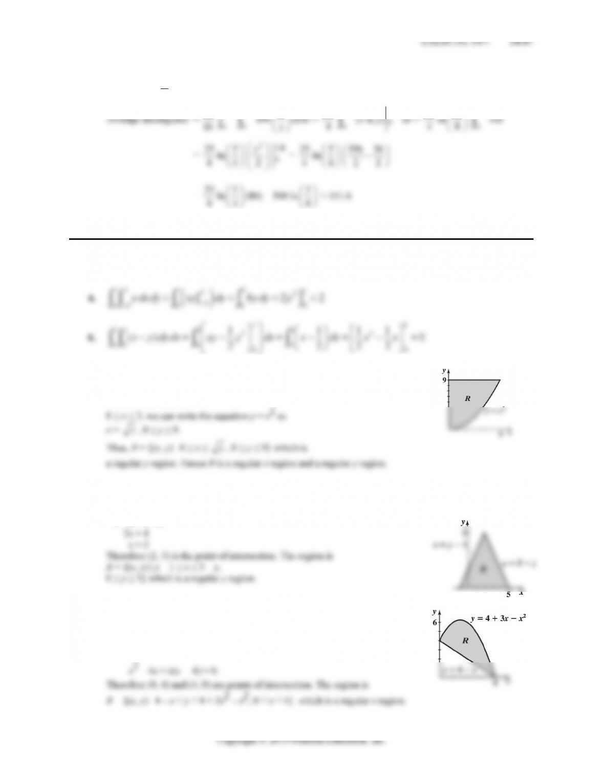
22. R = {(x, y) | 0 ≤ y ≤ 9 – x2, –3 ≤ x ≤ 3}
R
2x2y dA =
3
3
92
0
2
2
x
x
ydy
dx =
3
3
22 9
0
2
()
x
xy
dx =
3
3
[x2(9 – x2)2]dx
3
3
7
35
18
x
3
24. R = {(x, y) | y2 – 4 ≤ x ≤ 4 – 2y, 0 ≤ y ≤ 2}
A
(2x + 3y) dA =
2
0
42
4
2(2 3 )
y
y
x
ydx
dy =
2
0
42
2
4
2
(3)
y
y
xxy
dy
2
26. R = {(x, y) | 0 ≤ x ≤ 2
4yy, 0 ≤ y ≤ 2}
x
x
2
4
2
yy xdx
Letting u = 22
x
y holding y constant, we get du = 22
x
x
EXERCISE 14-7 14-39
Thus,
22
x
x
ydx =
du = u + C = 22
x
y + C
Therefore,
x
2
2
2
3(2)3/2 – 1
2(2)2 = 82
3 – 2
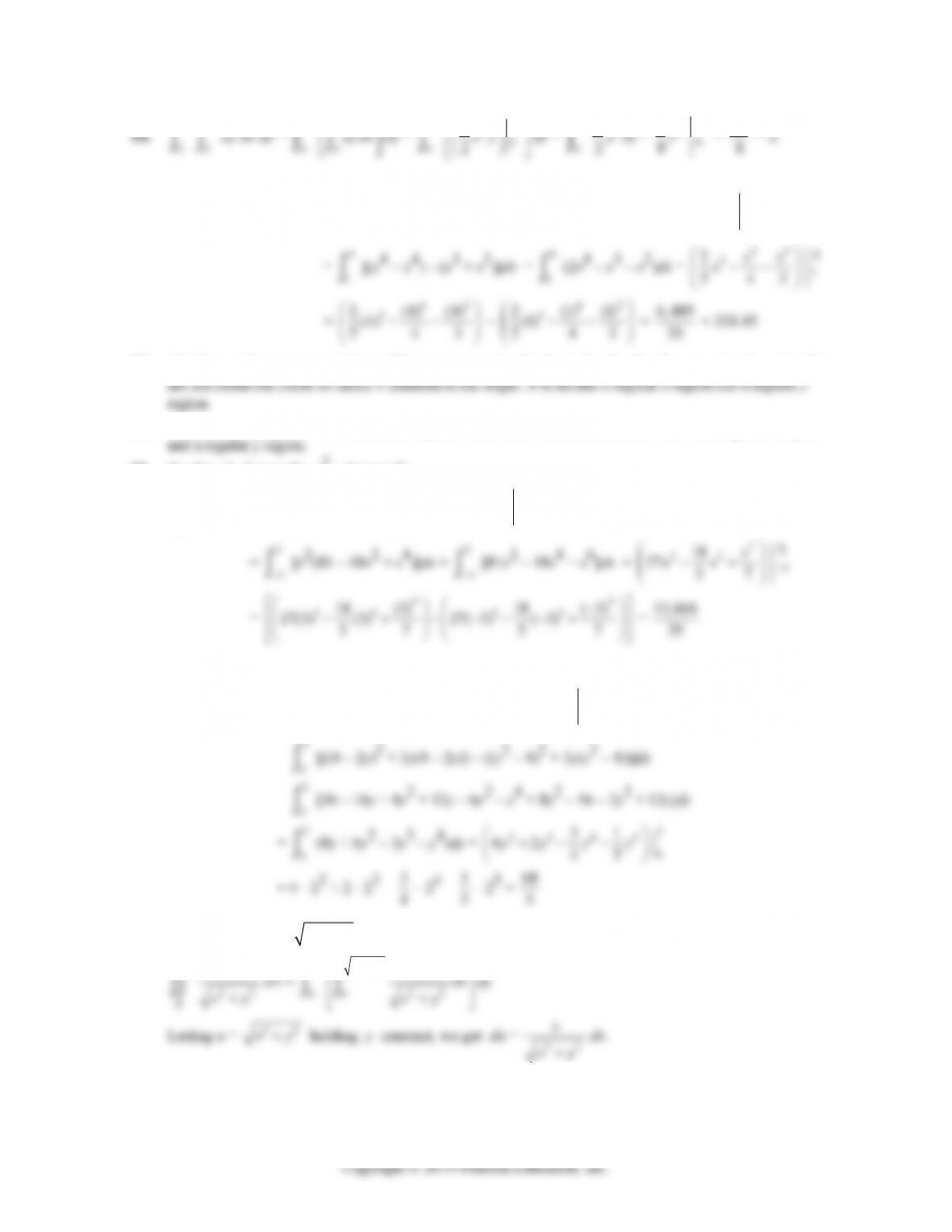
28. R = {(x, y) | x2 ≤ y ≤
x
, 0 ≤ x ≤ 1}
12xy dA =
1
0
212
x
x
x
ydx
dx
1
= (2x3 – x6)0
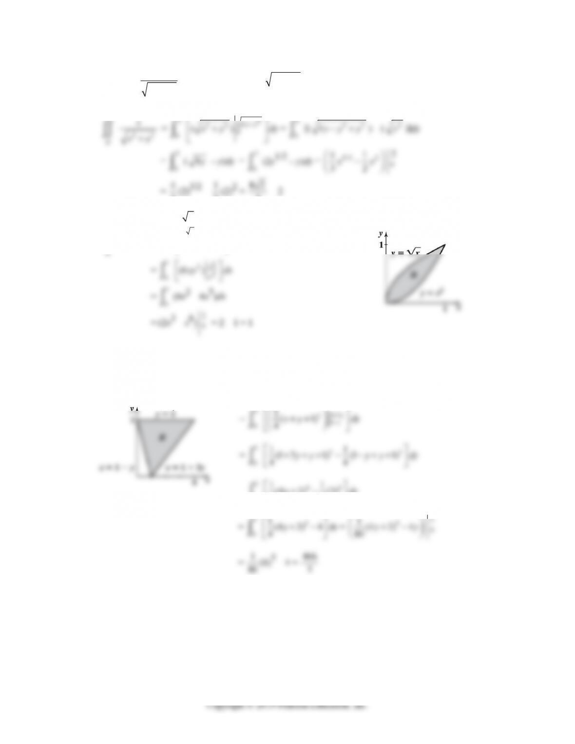
30. R = {(x, y) | 1 – y ≤ x ≤ 1 + 3y, 0 ≤ y ≤ 1}
R
(x + y + 1)3 dA =
1
0
13 3
1
(1)
y
y
x
ydx
dy
1
=
0
(4 2) (2)
44
y
dy
1
1