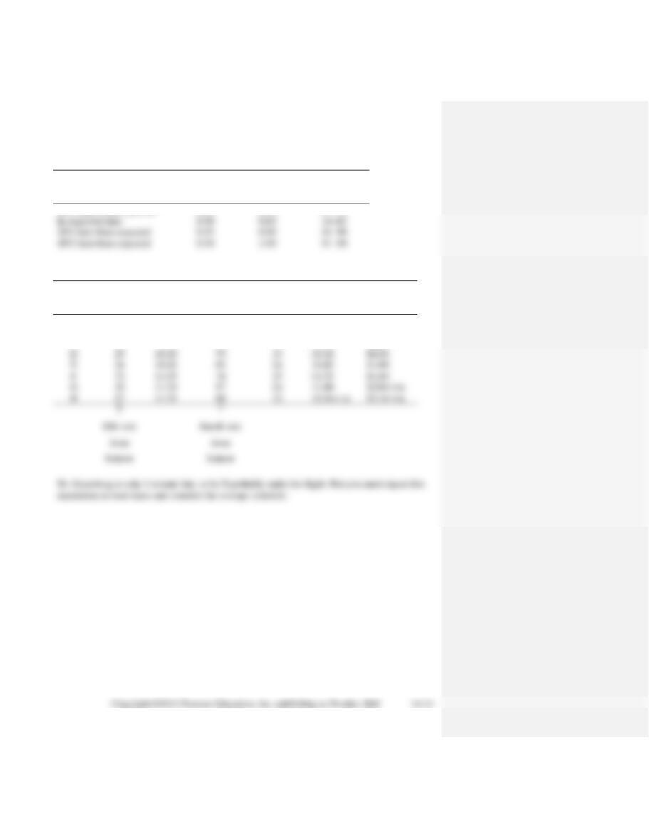
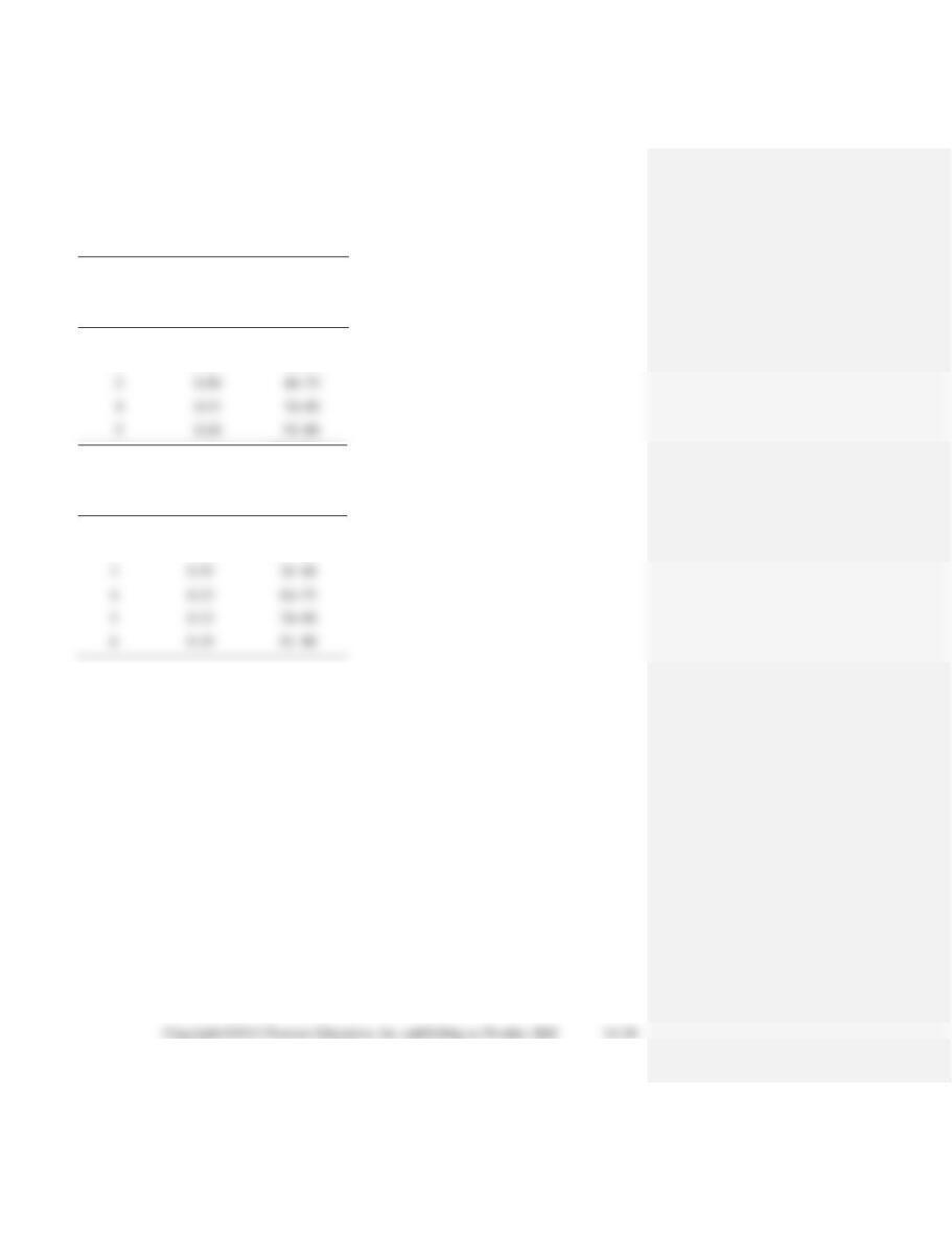
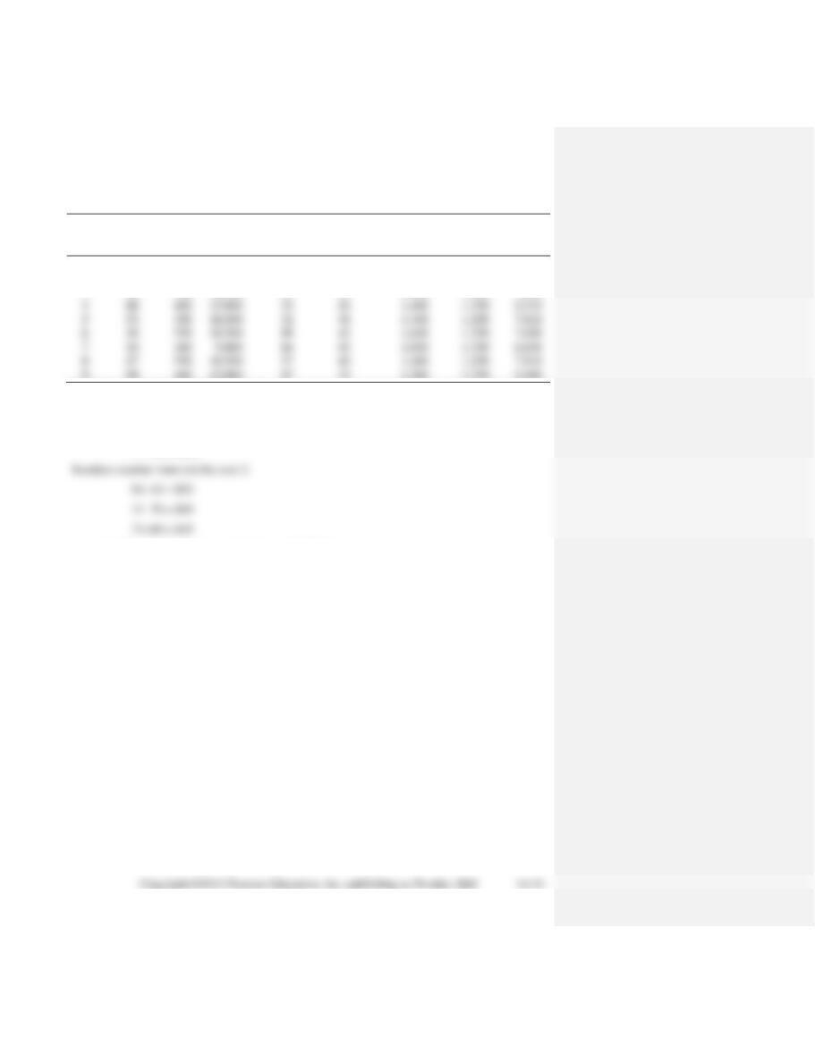
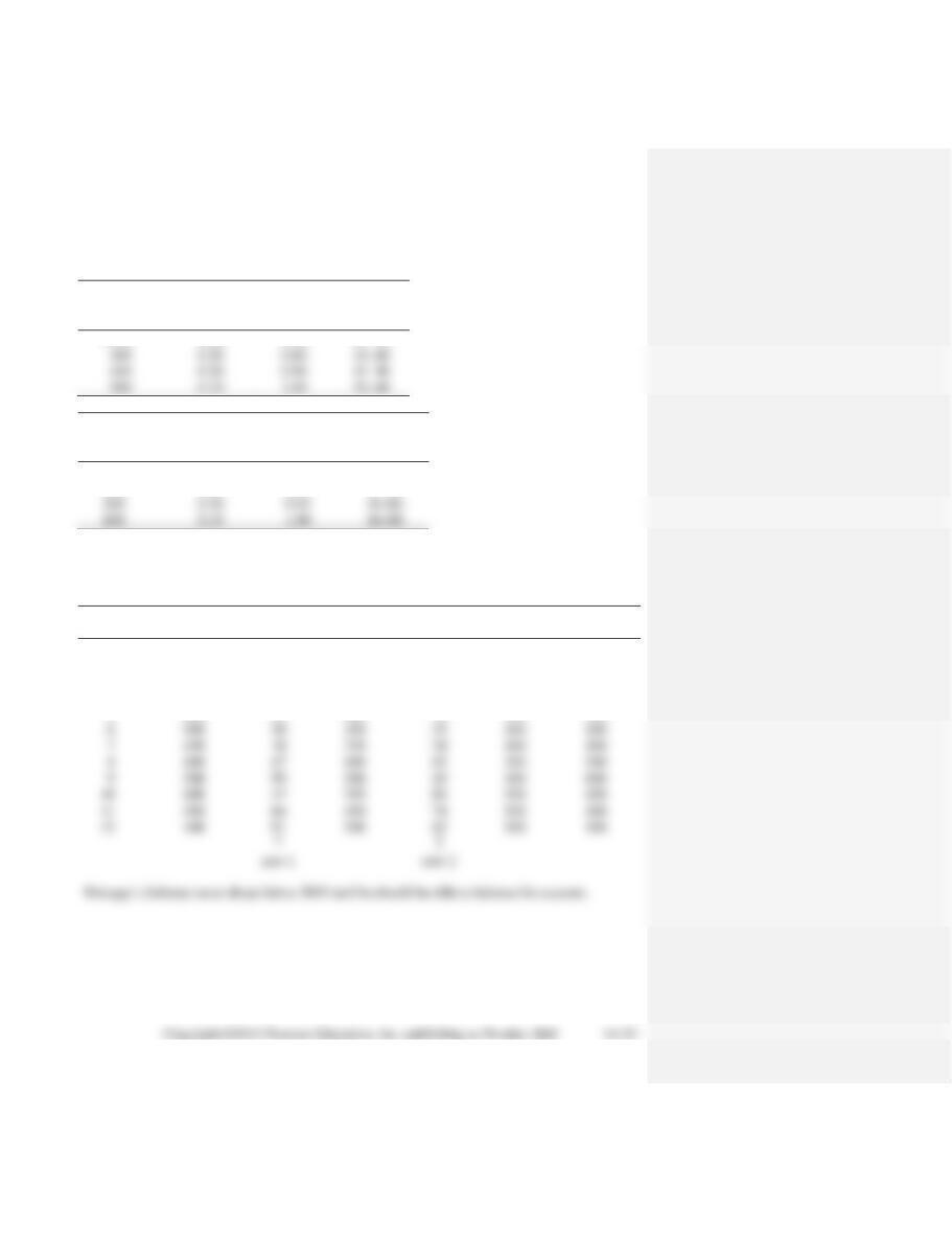
Random
Exam Time
Cumulative
Number
Distribution
Probability
Probability
Interval
20% faster than expected
0.15
0.15
01–15
1.00
91–00
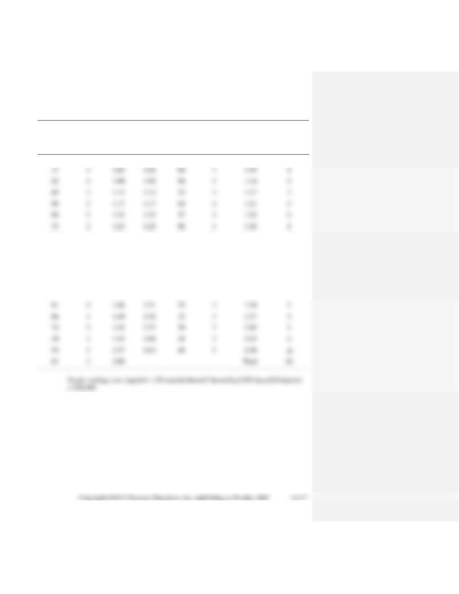
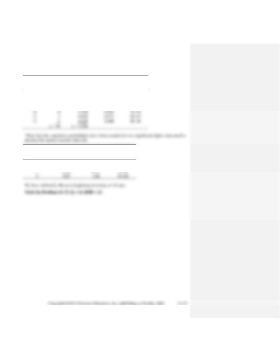
Table for 14-27.
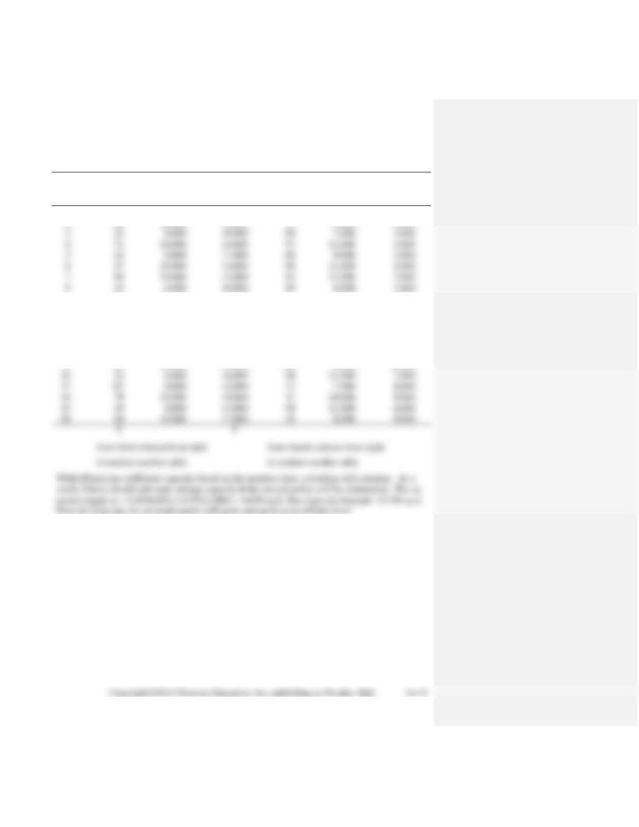
Arrival
Exam
Time
Time
Random
Time
Random
Length
In
Patient
Patient
Number
(A.M.)
Number
(Minutes)
(A.M.)
Leaves
A
60
9:30
80
18
9:30
9:48 A.M.
B
08
9:25
45
20
9:48
10:08
C
19
9:55
86
18
10:08
10:26
14
24
24
H
27
11:35
08
12

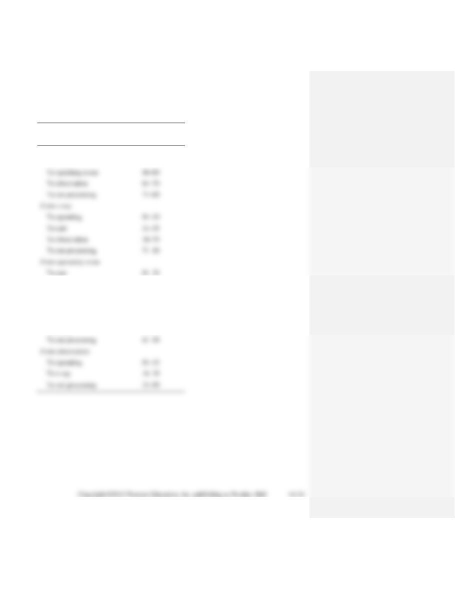
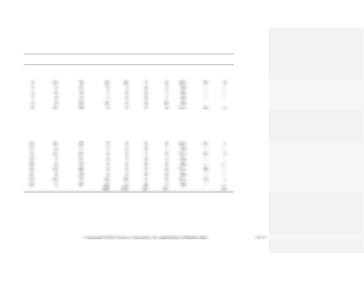
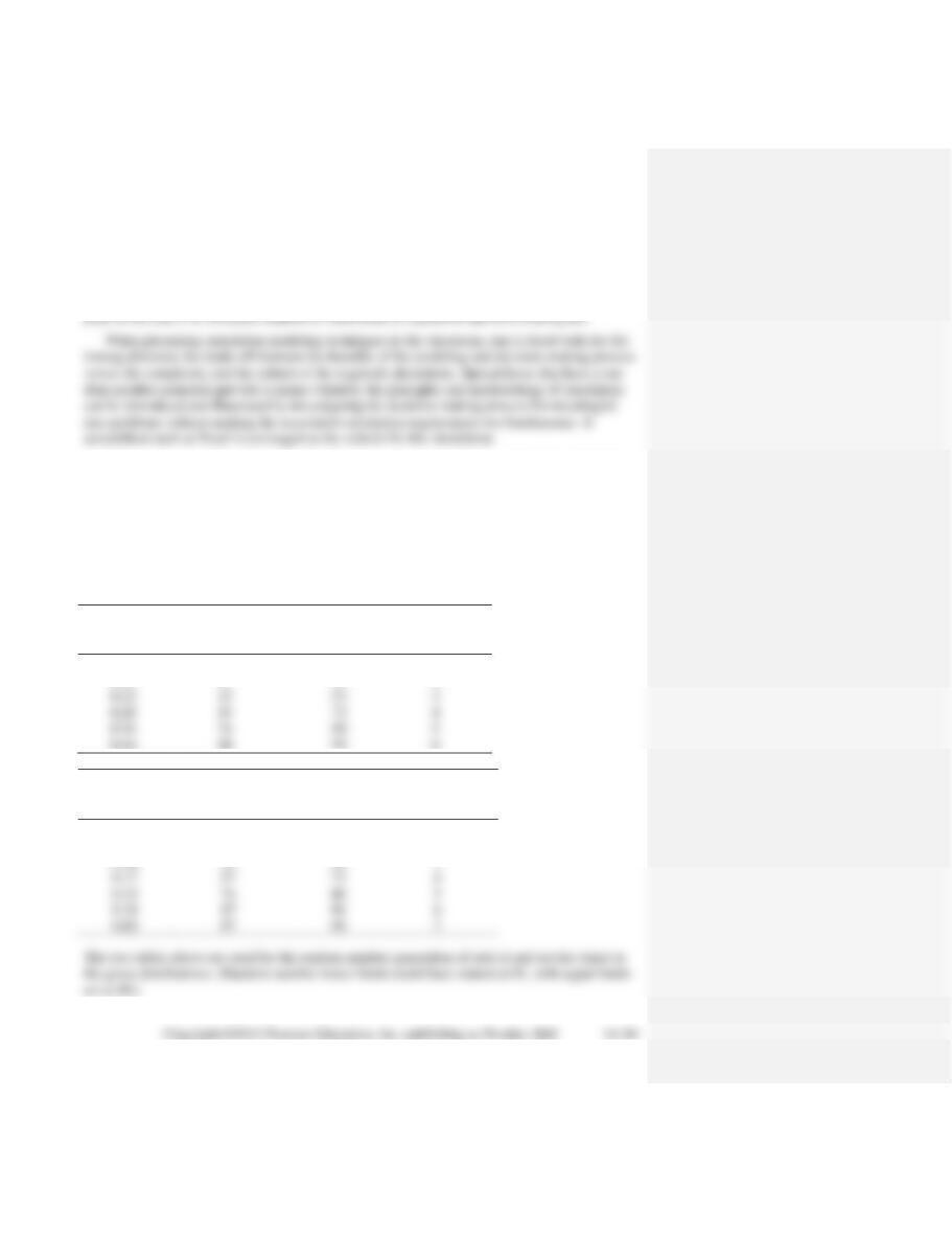
14–28. Actual distribution:
Random
Order
Cumulative
Number
(Sq. Ft.)
Probability
Probability
Interval
8,000
0.45
0.45
01–45
11,000
0.55
1.00
46–00
Demand distribution:
Steel per
Random
Week
Cumulative
Number
(Sq. Ft.)
Probability
Probability
Interval
6,000
0.05
0.05
01–05
7,000
0.15
0.20
06–20
8,000
0.40
0.70
10,000
0.90
1.00
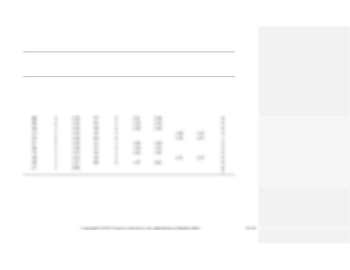
Sample Pelnor simulation for 20 weeks:
Size of
Inventory
End of
Random
Arriving
at Start
Random
Week
Week
Number
Shipment
of Week
Number
Demand
Inventory
1
84
11,000
11,000
00
11,000
0
2
55
11,000
11,000
59
9,000
2,000
25
10,000
09
7,000
3,000
71
11,000
14,000
97
11,000
3,000
34
11,000
69
9,000
2,000
57
11,000
13,000
98
11,000
2,000
7
50
11,000
13,000
93
11,000
2,000
9
95
11,000
12,000
51
9,000
3,000
10
64
11,000
14,000
92
11,000
3,000
11
16
8,000
11,000
92
11,000
0
12
46
11,000
11,000
16
7,000
4,000
13
54
11,000
15,000
84
10,000
5,000
14
64
11,000
16,000
27
8,000
8,000
15
61
11,000
19,000
64
9,000
10,000
16
23
18,000
94
7,000
18
79
11,000
19,000
71
10,000
9,000
19
19
8,000
17,000
94
11,000
6,000
20
50
11,000
17,000
30
8,000
9,000
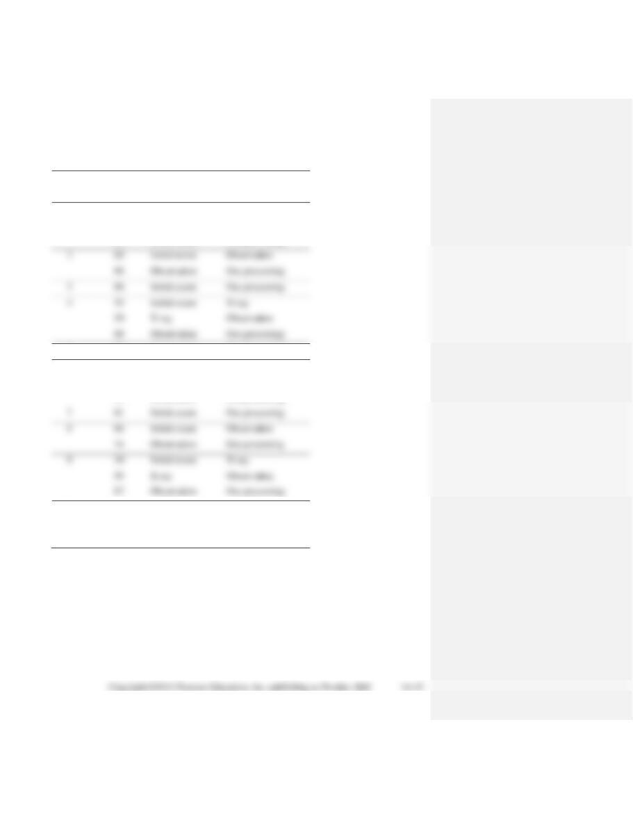
14–29. a. Random number intervals must be set for each from-to combination:
From-To
Random Number
Combination
Interval
From initial exam
To x-ray
01–45
To operating room
46–60
To observation
61–70
To out-processing
71–00
To operating
01–10
To observation
36–70
To out-processing
71–00
To cast
01–25
To observation
26–95
To out-processing
96–00
From cast fitting
To observation
01–55
To x-ray
56–60
To out-processing
61–00
To operating
01–15
To x-ray
16–30
Sample simulation using random numbers from Table 14.5, column 1:
Random
Person
Number
From
To
1
52
Initial exam
Operating room
37
Operating room
Observation
82
Observation
Out-processing
2
69
Initial exam
Observation
98
Observation
Out-processing
3
96
Initial exam
Out-processing
4
33
Initial exam
50
Observation
88
Observation
Out-processing
5
90
Initial exam
Out-processing
6
50
Initial exam
Operating room
27
Operating room
Observation
45
Observation
Out-processing
7
81
Initial exam
Out-processing
8
66
Initial exam
Observation
74
Observation
Out-processing
9
30
Initial exam
59
Observation
67
Observation
Out-processing
10
60
Initial exam
Operating room
60
Operating room
Observation
80
Observation
Out-processing
b. Using this very small simulation, no one goes to x-ray twice. It is very possible for this
situation to occur, however.
14–30.
Time
Random
Between
Number
Arrivals
Probability
Interval
1
0.20
01–20
2
0.25
21–45
3
0.30
46–75
4
0.15
76–90
5
0.10
91–00
Random
Service
Number
Time
Probability
Interval
1
0.10
01–10
2
0.15
11–25
3
0.35
26–60
4
0.15
61–75
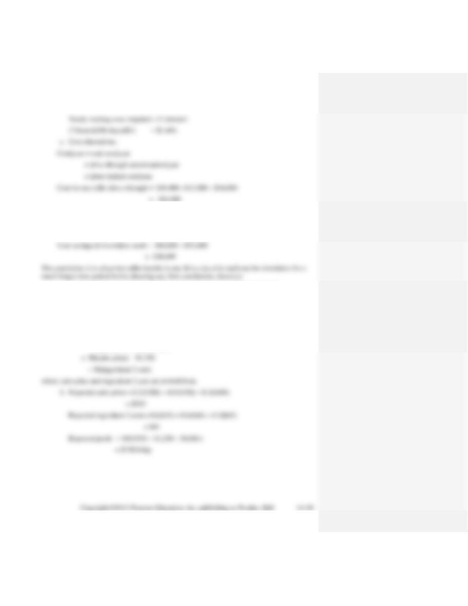
a. Simulation of one teller drive-through:
Time
Time
Wait
Random
Between
Actual
Service
Random
Service
Service
Time
Number
Arrivals
Time
Begins
Number
Time
Complete
(Minutes)
52
3
1:03
1:03
60
3
1:06
0
37
2
1:05
1:06
60
3
1:09
1
82
4
1:09
1:09
80
5
1:14
0
69
3
1:12
1:14
53
3
1:17
2
98
5
1:17
1:17
69
4
1:21
0
96
5
1:22
1:22
37
3
1:25
0
33
2
1:24
1:25
06
1
1:26
1
50
3
1:27
1:27
63
4
1:31
0
88
4
1:31
1:31
57
3
1:34
0
90
4
1:35
1:35
02
1
1:36
0
50
3
1:38
1:38
94
6
1:44
0
27
2
1:40
1:44
52
3
1:47
4
45
2
1:42
1:47
69
4
1:51
5
81
4
1:46
1:51
33
3
1:54
5
66
3
1:49
1:54
32
3
1:57
5
74
3
1:52
1:57
30
3
2:00
5
30
2
1:54
2:00
48
3
2:03
6
59
3
1:57
2:03
88
5
2:08
67
3
2:00
b. Simulation of two drive-through windows:
Service
Service
Service
Service
Starts
Ends
Starts
Ends
Time
At
At
At
At
Wait
Random
Between
Actual
Random
Service
Window
Window
Window
Window
Time
Number
Arrivals
Time
Number
Time
1
1
2
2
(Minutes)
52
3
1:03
60
3
1:03
1:06
0
37
2
1:05
60
3
1:05
1:08
0
82
4
1:09
80
5
1:09
1:14
0
69
3
1:12
53
3
1:12
1:15
0
98
5
1:17
69
4
1:17
1:21
0
96
5
1:22
37
3
1:22
1:25
0
33
2
1:24
06
1
1:24
1:25
0
50
3
1:27
63
4
1:27
1:31
0
88
4
1:31
57
3
1:31
1:34
0
90
4
1:35
02
1
1:35
1:36
0
50
3
1:38
94
6
1:38
1:44
0
27
2
1:40
52
3
1:40
1:43
0
45
2
1:42
69
4
1:43
1:47
1
81
4
1:46
33
3
1:46
1:49
0
66
3
1:49
32
3
1:49
1:52
0
74
3
1:52
30
3
1:52
1:55
0
30
2
1:54
48
3
1:54
1:57
0
59
3
1:57
88
5
1:57
2:02
0
67
3
2:00
0
1
Cost for two drive-throughs = $1,400 + $20,000
+ $32,000
= $53,400
SOLUTIONS TO INTERNET HOMEWORK PROBLEMS
14–31. a. Profit = (amount produced)(sales price)
– (ingredient 1 cost)(ingredient 1 units)
– (ingredient 2 cost)(ingredient 2 units)
= 30(sales price) – $50(25 units)
– (ingredient 2 cost)(36 units)
c.
Daily
Random
Sales
Gross
Random
Ingred. 2
Ingred. 2
Ingred.
Day
Number
Price
Sales
Number
Cost/Unit
Cost Total
1 Cost
Profit
1
52
$350
10,500
37
$40
$1,440
$1,250
$7,810
2
06
300
9,000
66
40
1,440
1,250
6,310
3
50
350
10,500
91
45
1,620
1,250
7,630
8
47
350
10,500
40
1,440
1,250
7,810
9
99
400
12,000
07
35
1,260
1,250
9,490
Random number intervals for sales price:
01–20 = $300
21–70 = $350
71–00 = $400
d. Expected profit from simulation = $7,770/day
14–32.
Demand
Random*
For
Fre
Cumulative
Number
Mercedes
quency
Probability
Probability
Interval
6
3
0.083
0.083
01–08
7
4
0.111
0.194
09–19
8
6
0.167
0.361
20–36
9
12
0.333
0.694
37–69
11
1
0.028
0.972
12
0.028
1.000
98–00
Random
Lead Time
Cumulative
Number
(Months)
Probability
Probability
Interval
1
0.44
0.44
01–44
2
0.33
0.77
45–77
Time
Beginning
Random
End
Lost
Place
Random
Lead
Period
Inventory
Number*
Demand
Sold
Inventory
Sale
Order
Number
Time
1
14
07
6
6
8
0
Yes
60
2
2
8
77
10
8
0
2
No
—
—
3
0
49
9
0
0
9
No
—
—
4
14
76
10
10
4
0
Yes
95
4
5
4
51
9
4
0
5
No
—
—
6
0
16
7
0
0
7
No
—
—
7
0
14
7
0
0
7
No
—
—
8
0
85
10
0
0
10
No
—
—
9
14
59
9
9
5
0
Yes
85
3
10
5
40
9
5
0
4
No
—
—
11
0
42
9
0
0
9
No
—
—
12
0
52
9
0
0
9
No
—
—
13
14
39
9
9
5
0
Yes
73
2
14
5
89
10
5
0
5
No
—
—
15
0
88
10
0
0
10
No
—
—
16
14
24
8
8
6
0
Yes
01
1
17
6
11
7
6
0
1
No
—
—
18
14
67
9
9
5
0
Yes
62
2
19
5
51
9
5
0
4
No
—
—
20
0
33
8
0
0
8
No
—
—
21
14
08
6
6
8
0
Yes
40
1
22
8
29
8
8
0
0
No
—
—
23
14
75
10
10
4
0
Yes
33
1
24
4
95
No
—
—
45
97
16
*Random numbers taken from column 18 of Table 14.5, reading top to bottom, then from column 17, reading bottom to top, alternat-
ing between Demand and Lead Time.
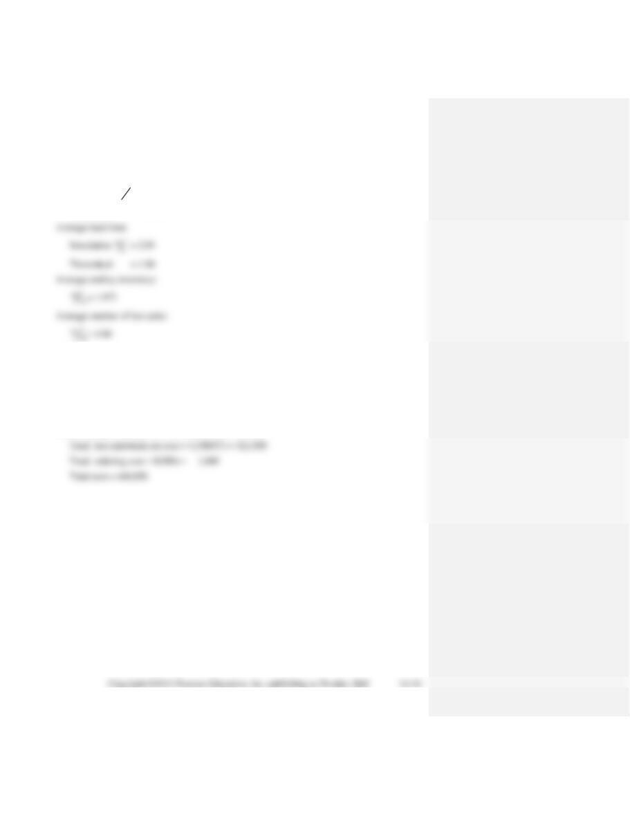
Useful statistics from the simulation:
Average demand:
Simulation
209 24
= 8.71
Theoretical = 8.75
4524
97 24
14–33. Total holding/carrying cost = 24(600)(1.875) = 27,000
Total lost sale/stock out cost = 4,350(97) = 421,950
Total ordering cost = 8(570) = 4,560
Total cost = 453,510 or $18,896 per month
14–34. Using the results from Problem 14-32, we have
Total holding/carrying cost = 24(500)(1.875) = 22,500
14–35.
Maruggi’s Solution
Cumul
Random
Maruggi’s
Proba
Proba
Number
Income
bility
bility
Interval
$350
0.40
0.40
01–40
400
0.20
0.60
41–60
450
500
0.10
1.00
91–00
Cumul
Random
Maruggi’s
Proba
Proba
Number
Expenses
bility
bility
Interval
$300
0.10
0.10
01–10
400
0.45
0.55
11–55
500
0.30
0.85
56–85
600
In this problem, students may select their own random numbers. If the instructor prefers, he or
she may assign rows 1 and 2 as we have used on the following page.
Beginning
Random
Random
Ending
Month
Balance
Number
Income
Number
Expense
Balance
1
$600
52
$400
37
$400
$600
2
600
06
350
63
500
450
3
450
50
400
28
400
450
4
450
88
450
02
300
600
5
600
53
400
74
500
500
6
500
30
350
35
400
450
8
400
47
400
03
300
500
37
60
450
66
450
74
500
400
400
91
500
85
500
400
SOLUTION TO ALABAMA AIRLINES CASE
This case describes a single-server queuing scenario that is to be investigated by simulation. The
basic premise can be applied to various queuing scenarios (e.g., bank, post office, cinema box
office, among others) and is not restricted to the Alabama Airlines reservation scenario. The pur-
In the assignment the students consider themselves to be quantitative analysts investigating
the particular scenario for their client(s). The assignments are presented in the form of a report to
their clients. For each scenario, an “executive summary” is required stating the main results and
recommendations. The body of the report then supports these recommendations with precise ex-
planations, relevant data, and models. Students are encouraged to be concise and to the point.
A spreadsheet model for the scenario should be constructed consisting of the following
items:
Arrival Interval Distribution
Random Number
Range
Lower
Upper
Arrival
Probability
Limit
Limit
Gap (Minutes)
0.11
00
10
1
0.21
11
31
2
0.22
32
53
3
73
0.16
74
89
5
0.10
90
99
6
Service Time Distribution
Random Number
Range
Lower
Upper
Service
Probability
Limit
Limit
Time (Minutes)
0.20
00
19
1
0.19
20
38
2
0.18
39
56
3
0.17
57
73
4
0.13
74
86
5
0.10
87
96
6