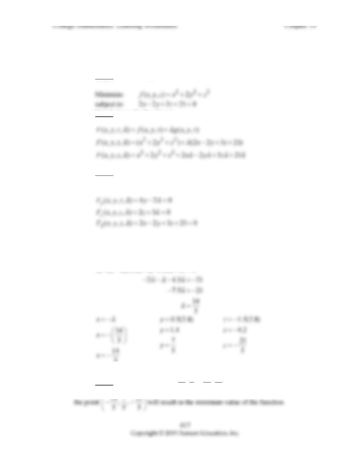
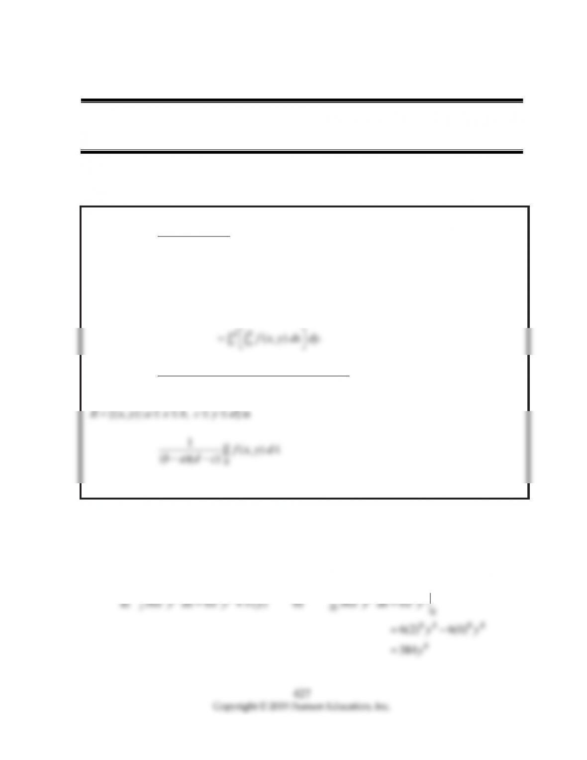
4. Minimize: 222
(, ,) 2
f
xyz x y z
subject to: 223 21xyz
Step 1: Rewrite the problem.
f
Step 2: Form the function F.
Step 3
: Find the critical points.
(, ,, ) 2 2 0
x
Fxyz x
λλ
Therefore, ,x
λ
0.5 ,y
λ
and 1.5 .z
λ
223210
2( ) 2(0.5 ) 3( 1.5 ) 21 0
xyz
λλ λ
5
Step 4: Since the solution 14 7 21 14
,, ,
55 5 5
is the only critical point of F,

418
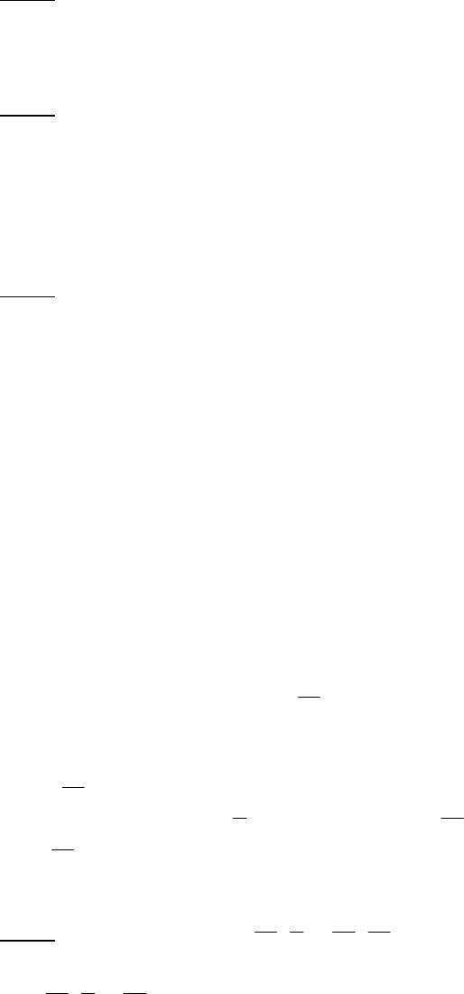
5. Maximize: ( , , ) 5
f
xyz xyz
subject to: 3 2 3 90xyz
Step 1
: Rewrite the problem.
f
Step 2
: Form the function F.
Step 3
: Find the critical points.
(, ,, ) 5 3 0
x
Fxyz yz
λλ
Simplifying the first two equations will yield the result 1.5
y
xand simplifying the
first and third equations will yield the result .zx
323900
xyz
1.5
y
x
zx
530
yz
λ
Step 4: Since the solution
10,15,10, 250is the only critical point of F, the
point
10,15,10 will result in the maximum value of the function.

College Mathematics: Learning Worksheets Chapter 14
419
Name ________________________________ Date ______________ Class ____________
Goal: To find the equation of a line using the method of least squares
Section 14-5 Method of Least Squares
Theorem: Least Squares Approximation
For a set of n points 11 2 2
( , ), ( , ), ( , ),
nn
x
yxy xyL the coefficients of the least squares
line yaxbare the solutions of the system of normal equations
2
111
nnn
kkkk
kkk
x
axbxy
x
and are given by the formulas
111
2
nnn
kk k k
kkk
nxy x y
a
College Mathematics: Learning Worksheets Chapter 14
420
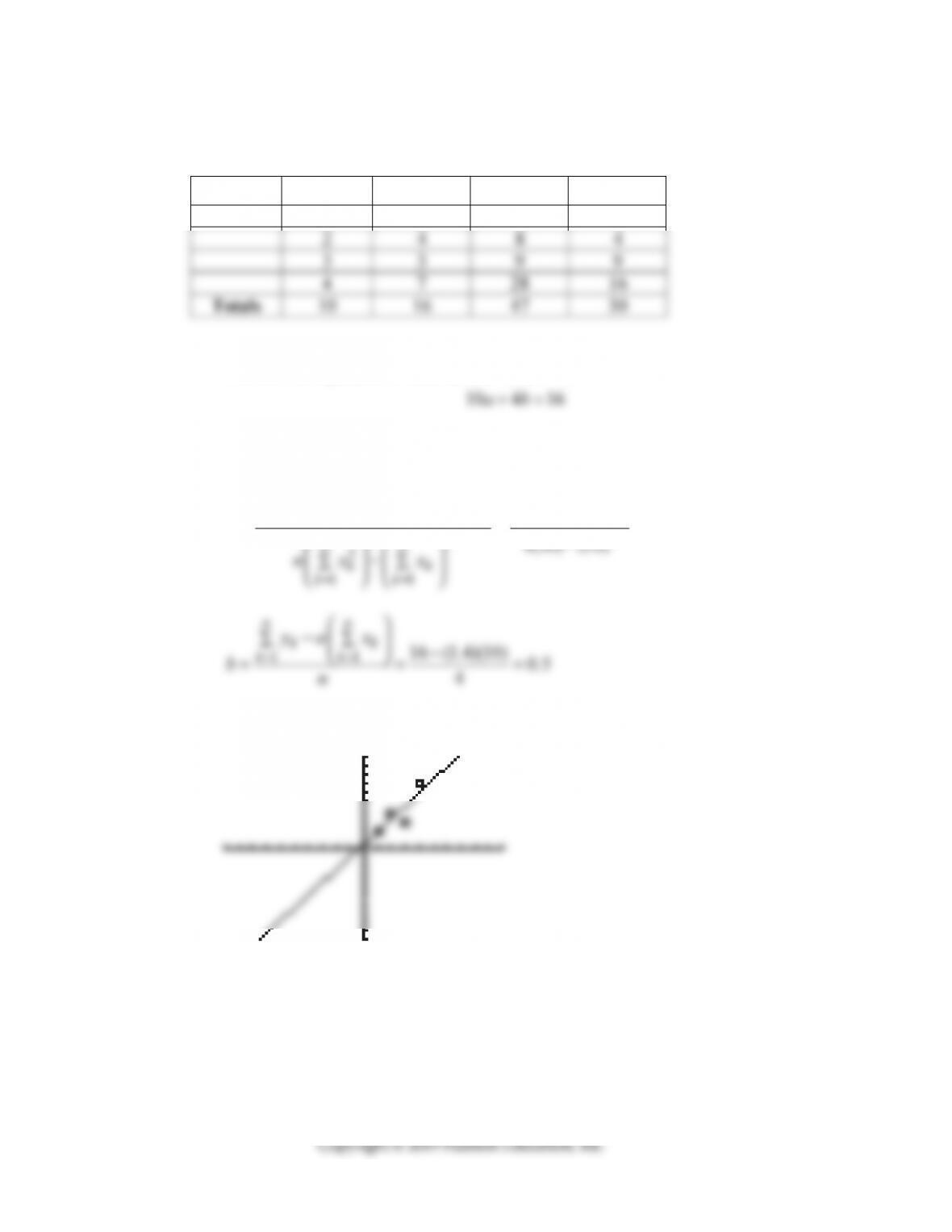
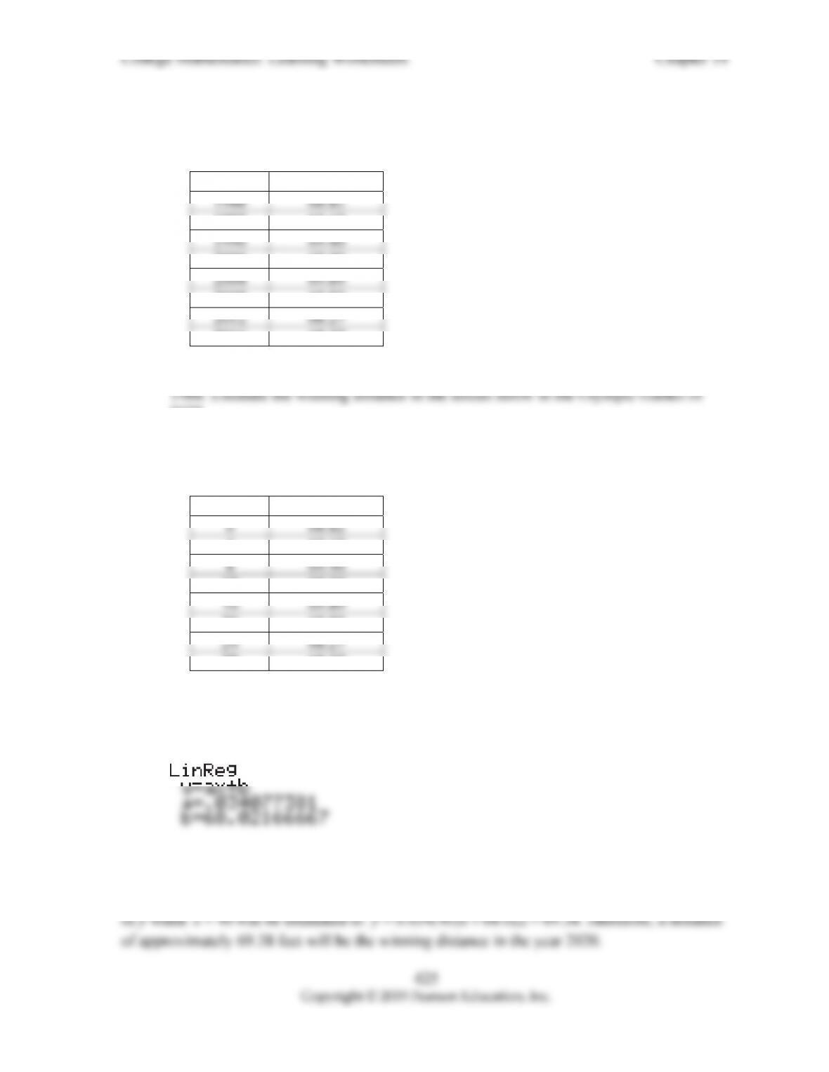
In Problems 1 and 2, find the least squares line. Graph the data and the least squares line.
1.
x y xy 2
x
1 2 2 1
The normal equations would be 30 10 47
ab
+=
The solutions for a and b are
111
22
4(47) (10)(16) 1.4
nnn
kk k k
kkk
nxy x y
a
===
⎛⎞⎛⎞⎛⎞
−
∑∑∑
⎜⎟⎜⎟⎜⎟−
⎝⎠⎝⎠⎝⎠
===
Therefore, the equation of the least squares line is 1.4 0.5.yx=+
421
2.
x y xy 2
x
1 3 3 1
2 0 0 4
The normal equations would be 30 10 7
ab
The solutions for a and b are
111
4( 7) (10)(0) 1.4
nnn
kk k k
kkk
nxy x y
a
Therefore, the equation of the least squares line is 1.4 3.5.yx
422
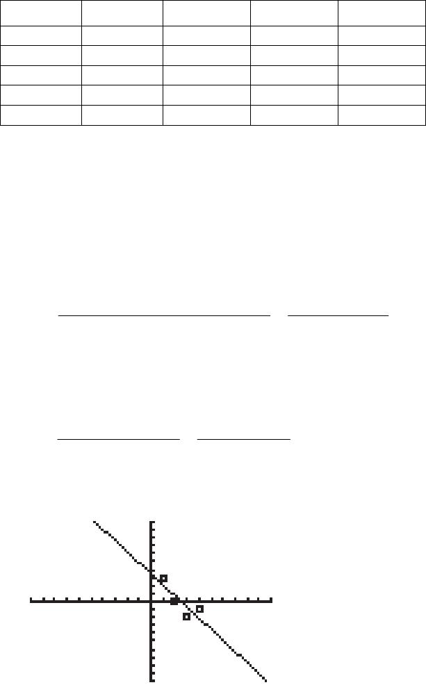
3.
x y xy 2
x
3 2 6 9
5 8 40 25
The normal equations would be 285 35 250
35 5 32
ab
ab
The solutions for a and b are
5(250) (35)(32) 0.65
nnn
kk k k
kkk
nxy x y
Therefore, the equation of the least squares line is 0.65 1.85yxand the value of y
423
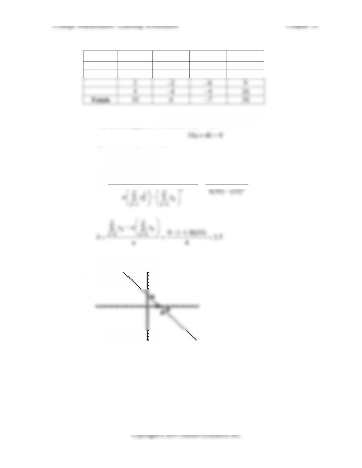
4.
x y xy 2
x
–3 9 –27 9
0 8 0 0
Estimate y when 9.x
The normal equations would be 90 0 78
ab
The solutions for a and b are
111
5( 78) (0)(35) 0.87
nnn
kk k k
kkk
nxy x y
a
Therefore, the equation of the least squares line is 0.87 7yx and the value of y
424
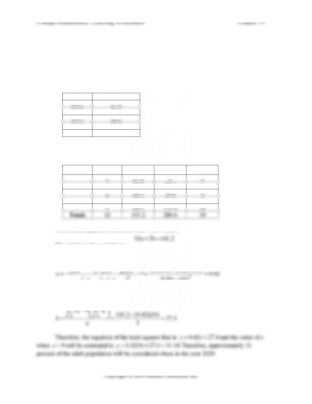
5. The U.S. Centers for Disease Control and Prevention (CDC) use a measure called
body mass index (BMI) to determine whether a person is obese. A BMI between 25.0
and 29.9 is considered overweight, and a BMI of 30.0 or more is considered obese.
The following table shows the percent of United States adults 18 years and older who
were obese in the years indicated, judging on the basis of BMI. (Source: CDC,
October 13, 2017)
Year Percent Obese
2012 27.7
2014 28.9
2015 28.9
Using 0 for 2011, find the least squares line and use it to predict the percent of adults
18 years and older that will be obese in the year 2020.
x y xy 2
x
1 27.7 27.7 1
3 28.9 86.7 9
The normal equations would be 30 10 286.6
ab
+=
The solutions for a and b are
2
11
5(30) (10)
nnn
kk k k
nn
kk
kk
nxy x y
nx x
==
⎛⎞⎛⎞⎛⎞
−
∑∑∑
⎜⎟⎜⎟⎜⎟ −
−
⎛⎞⎛⎞
−
∑∑
⎜⎟⎜⎟
⎝⎠⎝⎠
nn
⎛⎞
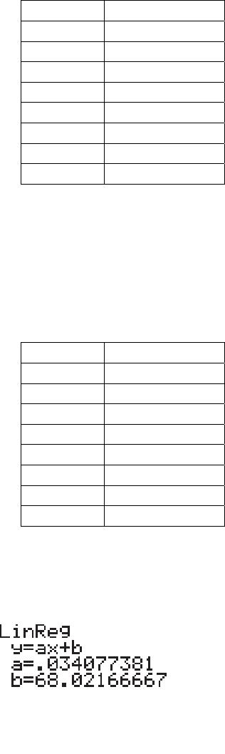
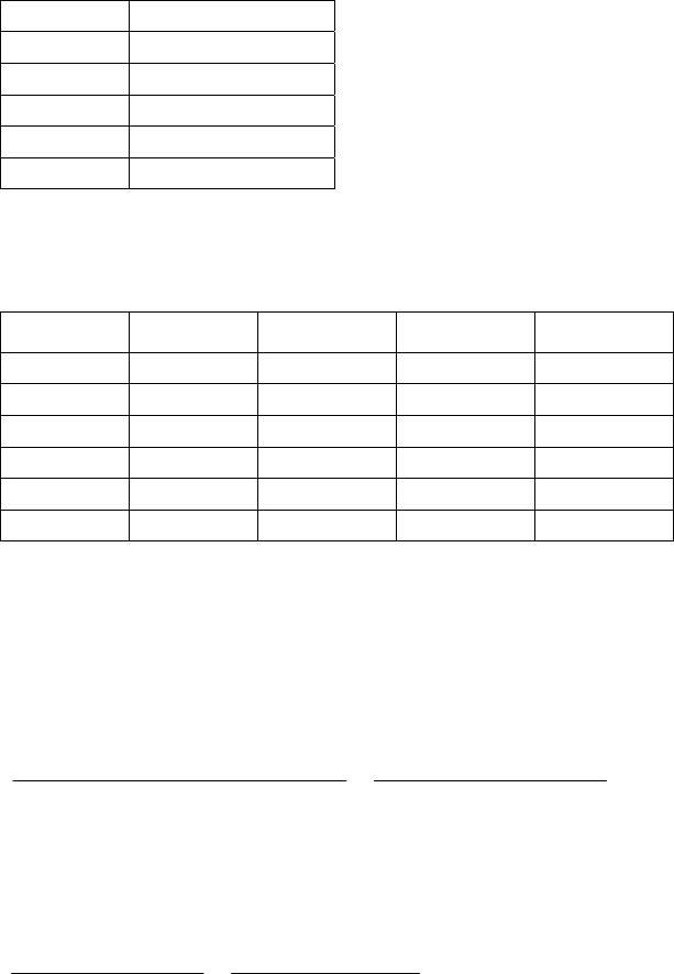
6. The table gives the winning distance in the discus throw in the Olympic Games from
1988 to 2016.
Year Distance (ft)
1992 65.12
2000 69.30
2008 68.82
2016 68.37
Use a graphing calculator to find the least squares line for the data, letting 0xfor
2028.
Rewrite the table using x for the year and y for the distance.
x Y
4 65.12
12 69.30
20 68.82
28 68.37
On your graphing calculator, go into the “STAT” mode and enter the x values to list 1
and the y values to list 2. Next go to the “CALC” mode within “STAT”. Option
number 4 is “LinReg(ax+b). Hit the enter key twice for the following result:
Therefore, the equation of the least squares line is 0.034 68.022yx=+and the value


College Mathematics: Learning Worksheets Chapter 14
426

College Mathematics: Learning Worksheets Chapter 14
Name ________________________________ Date ______________ Class ____________
Goal: To evaluate indefinite and definite double integrals
In Problems 1 and 2, find each antiderivative. Then use the antiderivative to evaluate the
definite integral.
1. a) 54
36
x
ydx
∫ b)
254
036
x
ydx
∫
x
254 64
Section 14-6 Double Integrals over
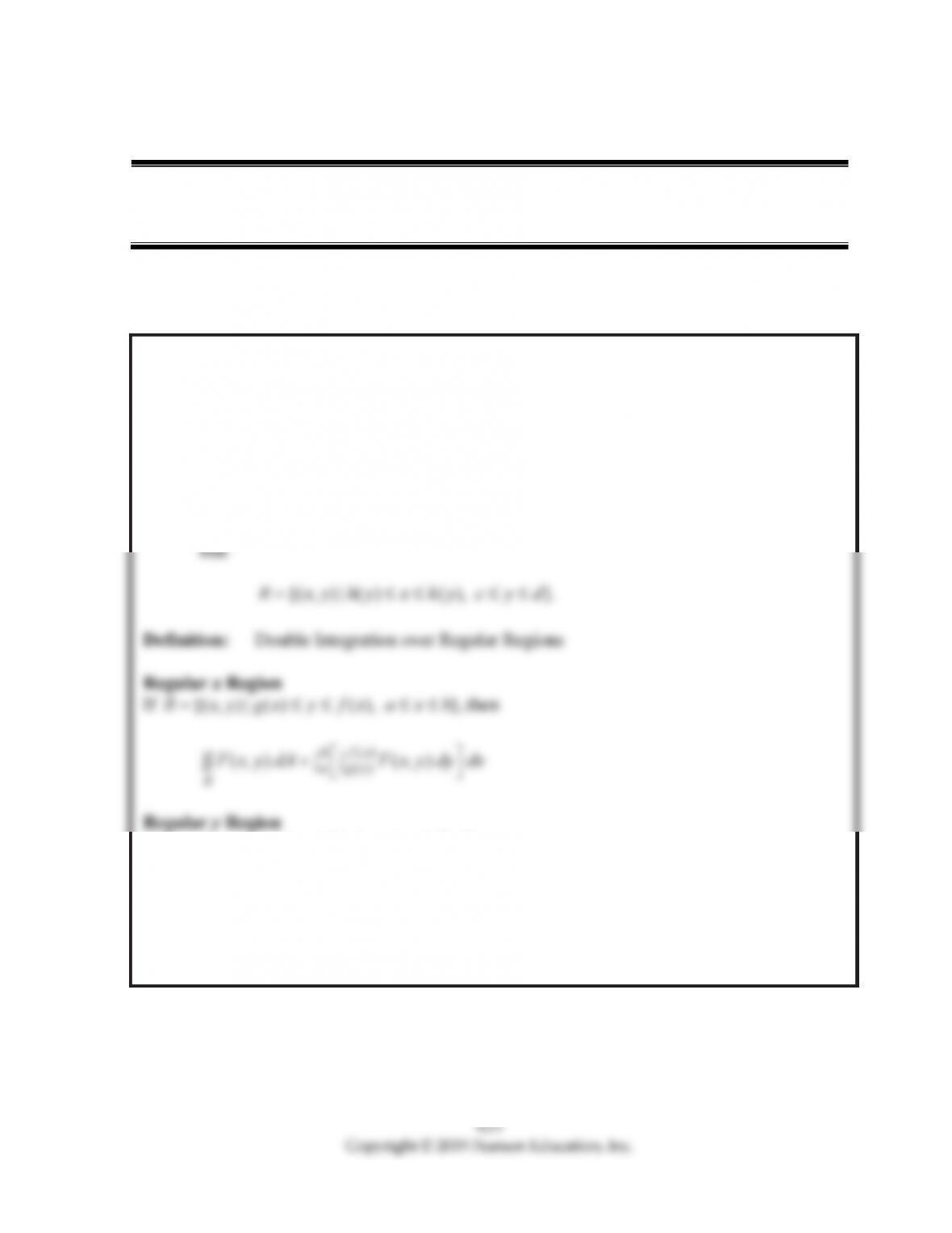
Rectangular Regions
Definition: Double Integral
The double integral of a function ( , )
f
xyover a rectangle
{( , ) | , }
R
xy a x b c y dis
(, ) (, )
bd
ac
R
f
xy dA f xy dy dx
f
Definition: Average Value over Rectangular Regions
The average value of the function ( , )
f
xyover the rectangle
College Mathematics: Learning Worksheets Chapter 14
2. a) 2
ln
x
dy
xy
b)
2
12
ln
x
dy
xy
2
x
x
x
3. 75
01
(8 6 7)
x
ydxdy
−++
∫∫
5
0
x
=
[]
7
0
7
138 36
ydy
=+
∫
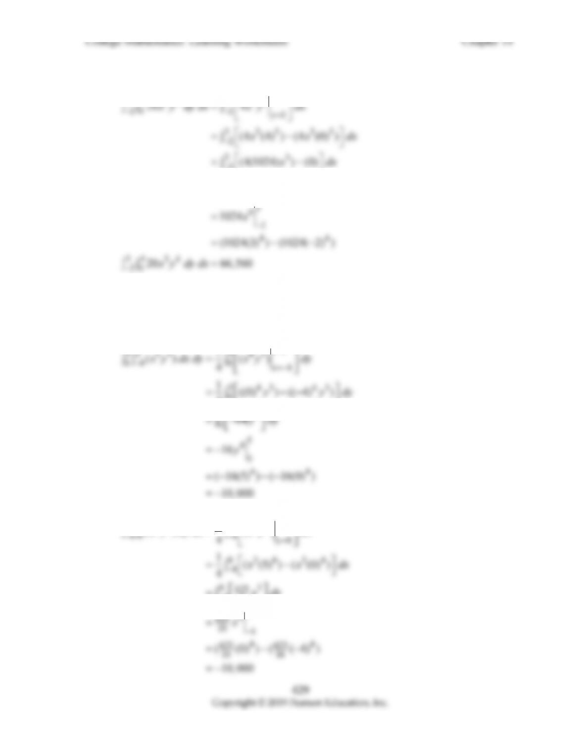
4. 34 34
20
20
x
ydydx
34 3
34 35
2
y
x
33
2
4096
xdx
5. Use both orders of iteration to evaluate the double integral.
33
();
R
x
ydA
{( , ) | 4 0, 0 5}Rxy x y=−≤≤≤≤
0
0
53
4
x
=
⎡⎤
5
05 0
33 34
44
0
1
() ()
y
x y dy dx x y dx
xdx
=
−
⎡⎤
=
=∫⎣⎦
6. Find the average value of the function over the given rectangle.
23
(, ) 3 4 ;
f
xy x y {( , ) | 0 4, 3 1}Rxy x y
13
(4 0)(1 ( 3)) 16
164 16
x
7. Find the volume of the solid under the graph of the function over the given rectangle.
(, ) 4 8 7;fxy x y {( , ) | 2 2, 1 3}Rxy x y
2
32 3 2
1
3
2
16 28
x
yy

College Mathematics: Learning Worksheets Chapter 14
Name ________________________________ Date ______________ Class ____________
Goal: To evaluate double integrals over non–rectangular regions
Section 14-7 Double Integrals over More
General Regions
Definition: Regular Regions
A region R in the xy plane is a regular x region if there exist functions f(x) and g(x)
and numbers a and b such that
{( , ) | ( ) ( ), }.
R
xy gx y f x a x b
A region R is a regular y region if there exist h(y) and k(y) and numbers c and d such
If {( , ) | ( ) ( ), },
R
xy hy x ky c y dthen
()
()
(, ) (, )
ky
d
chy
R
F x y dA F x y dx dy
432
1. Evaluate the following integral.
82
00
(3 )
x
x
ydydx+
∫∫
3
03
(3 )
yx
xdx
=
=+
∫
4
8
3
()
x
x
=+
2. Use the description of the region R to evaluate the integral.
(2 3) ;
R
x
ydA
{( , ) | 0 , 0 6}Rxy xy y
66
2
1
(2 3) (2 3)
xy
y
x y dx dy x y dy
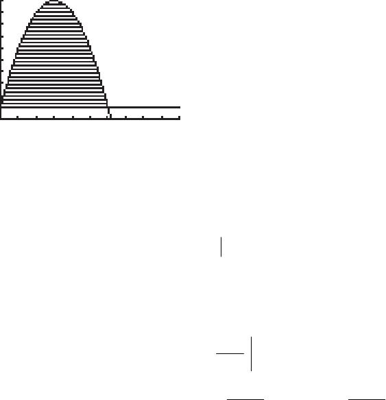
3. Graph the region R bounded by the graphs of the indicated equations. Describe R in
set notation with double inequalities, and evaluate the indicated integral.
2
16 ,
y
xx 1;y 15
R
x
dA
The region bounded by the equations is (the window shown is quadrant 1 only)
0
(90 15 )
x
xxdx
4
6
315
(30 )
x
x
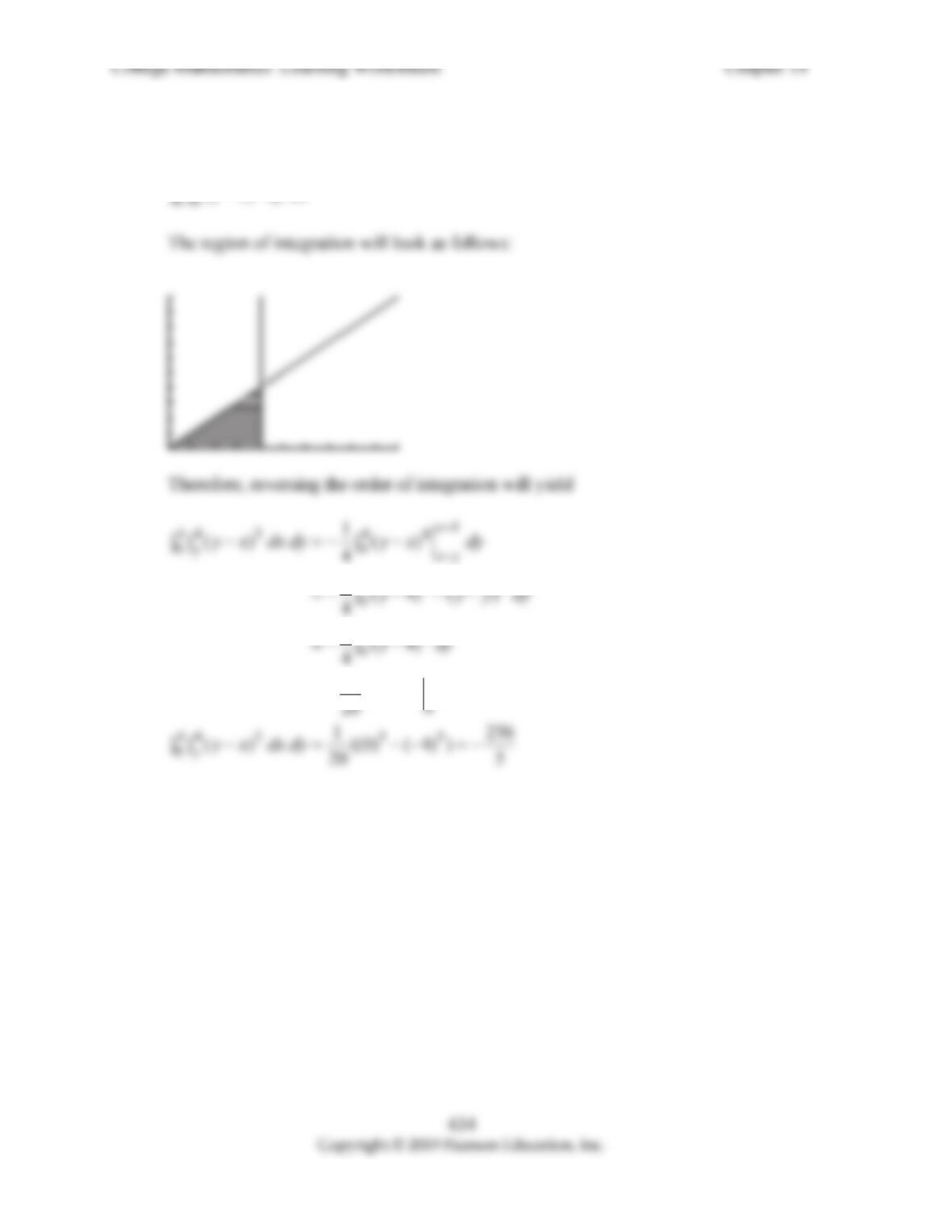
4. Graph the region of integration, reverse the order of integration, and then evaluate the
integral with the order reversed.
43
()
x
y
xdydx
444
44
1(4)( )
1(4)
4
5
1(4)
y
435
5. Reverse the order of integration and then evaluate the integral with the order reversed.
Do not attempt to evaluate the integral in the original form.
25 4 3
0(4)
y
x
dx dy
00 0 0
(4) 4
y
xdydxyx dx
32
3
0
1(4)
3
x
436
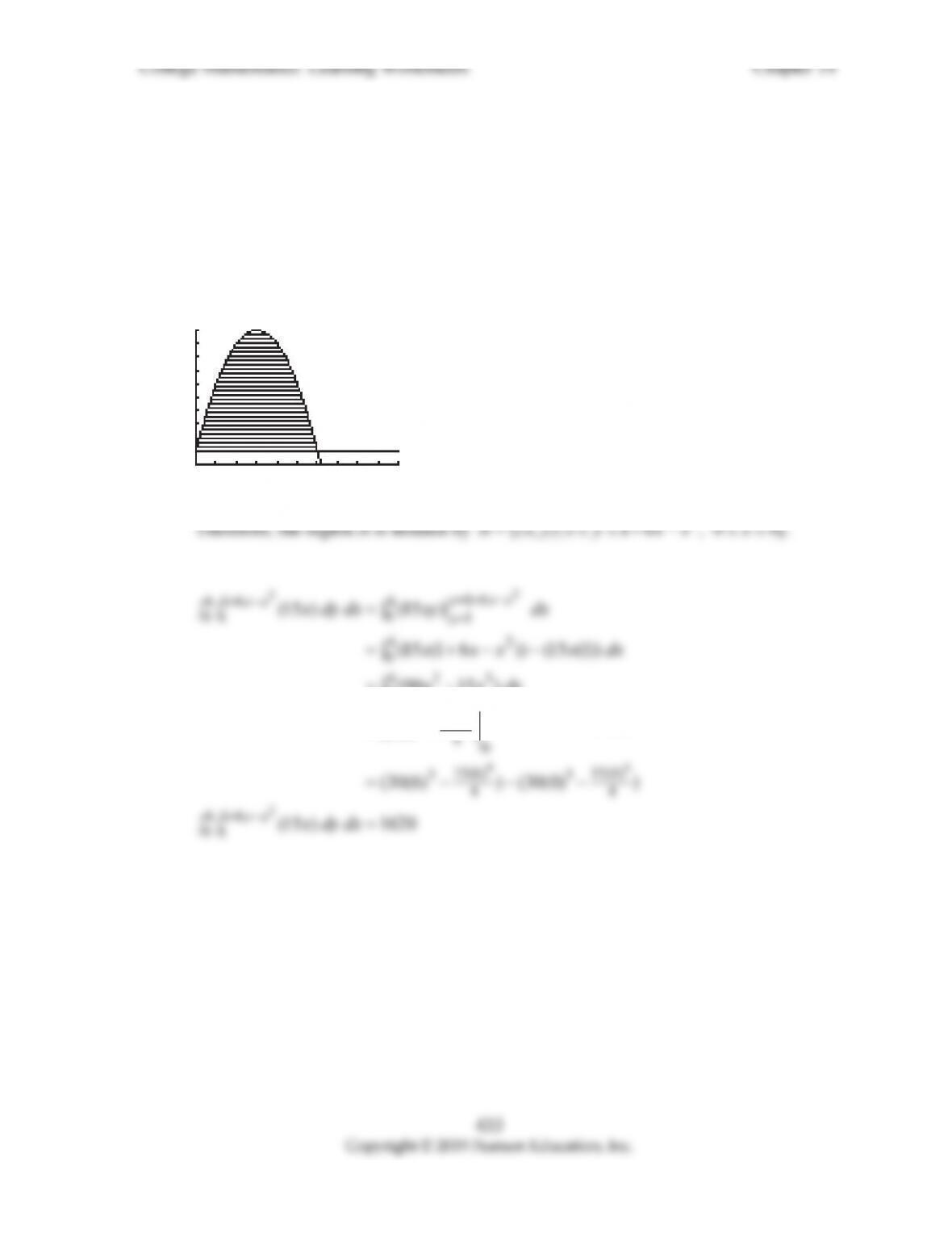
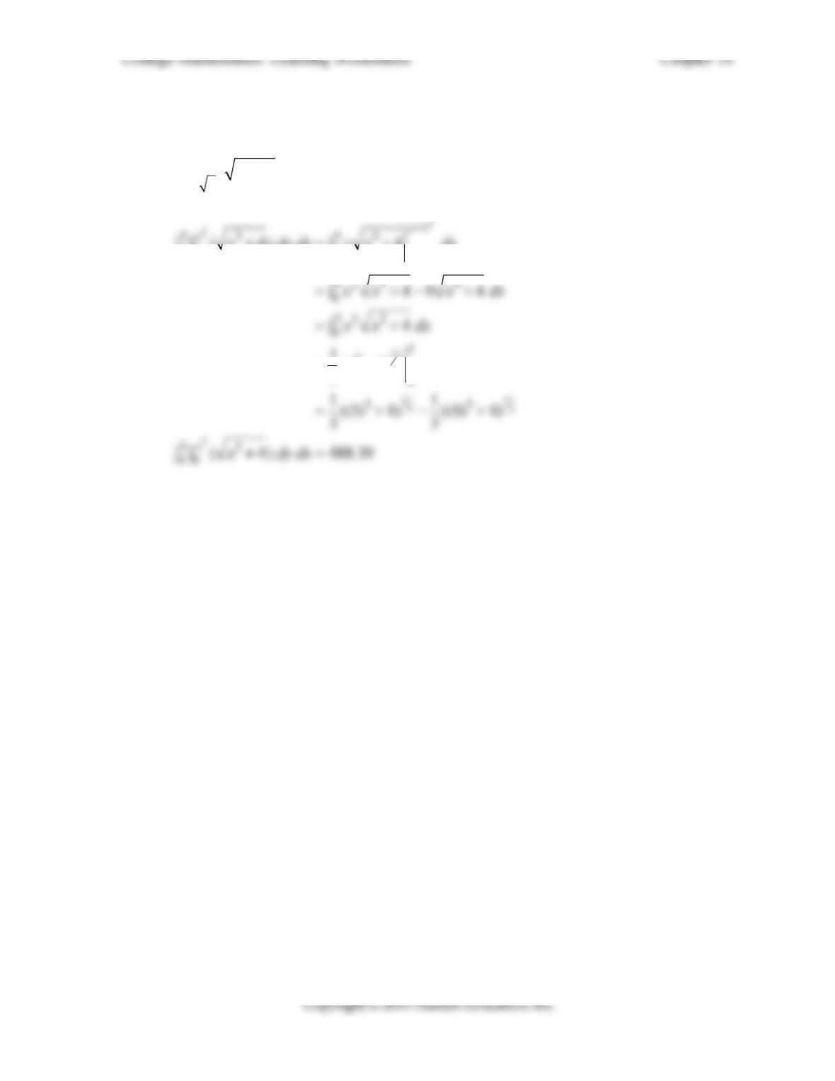
6. Use a graphing calculator to graph the region R bounded by the graphs of the
indicated equations. Use approximation techniques to find intersection points correct
to two decimal places. Describe R in set notation with double inequalities, and
evaluate the indicated integral correct to two decimal places.
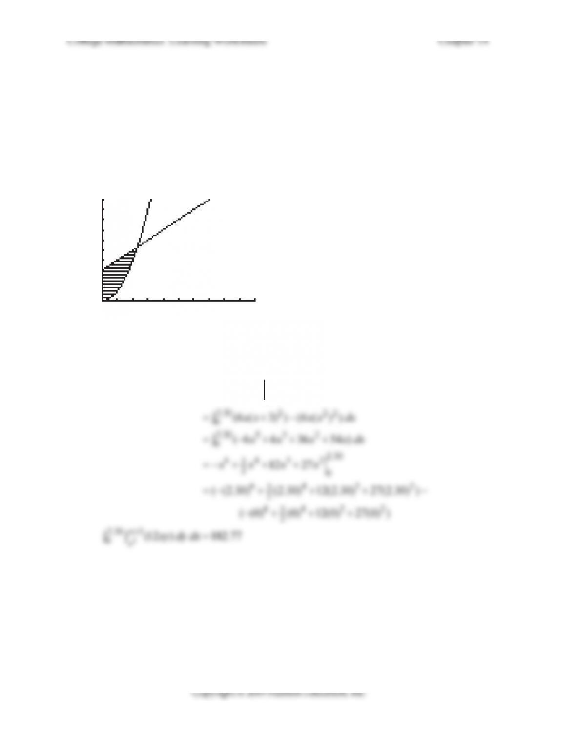
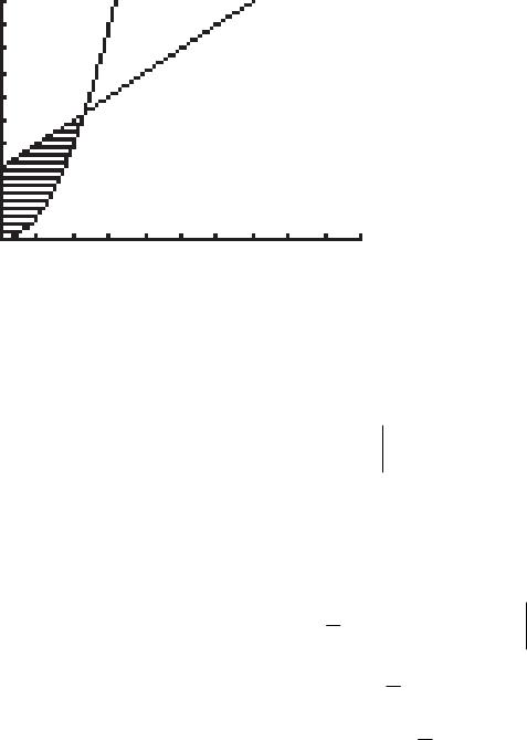
2
3, , 0;yx yx x 12
R
x
ydA
The region bounded by the above equations is as follows:
The point of intersection is found by using the intersect feature on the calculator. The
point of intersection is (2.30, 5.30). Therefore, the region of integration R is defined by
2
{( , ) | 3, 0 2.30}.Rxyxyx x
22
3
2.30 3 2.30 2
00
(12 ) (6 )
yx
x
xyx
xy dy dx xy dx