Chapter 13 – Inventory Management
13-21
P (stockout) = ?
21.208.
871.1
639.6
Z,solving =
−
=
22.
d = 30 gal./day
ROP = 170 gal.
LT = 4 days
ss = Zd LT = 50
ss = 50 gal.
Risk = 9% Z = 1.34
Solving, d LT = 37.31
3% Z = 1.88 x 37.31 = 70.14 gal.
24. SL 96% → Z = 1.75 ROP =
dLT
+ Z
2
LT
2
2
ddLT +
Chapter 13 – Inventory Management
13-22
25. LT = 3 days S = $30
D = 4,500 gal H = $3
Risk = 1.5% → Z = 2.17
a. Qty. Unit Price Qo =
300
H
DS2=
1 – 399 $2.00
400 – 799 1.70
800+ 1.62
b. ROP =
d
LT + Z
d
LT
= 12.5 (3) + 2.17
3
(2)
= 37.5 + 7.517
= 45.02 gal.
26. d = 5 boxes/wk.
d = .5 boxes/wk.
LT = 2 wk.
S = $2
b.
ROP =
d
(LT) + z
LT
(d)
83.2
)5(.2
)2(512
)(LT
)LT(dROP
z
d
=
−
=
−
=
Thus,
Chapter 13 – Inventory Management
13-23
27.
d
= 80 lb.
d= 10 lb.
LT
= 8 days
LT = 1 day
SL = 90 percent, so z = +1.28
28.
D = 10 rolls/day x 360 days/yr. = 3,600 rolls/yr.
d
= 10 rolls/day
LT = 3 days
H = $.40/roll per yr.
d = 2 rolls/day
S = $1
a.
0
2 2(3,600)1 134.16
.40
DS
QH
= = =
b.
SL of 96 percent requires z = +1.75
[round to 134]
d.
000413.
16.134
464.3
)016(.)(1
==
=−
dLT
annual
Q
zESL
d
= 748.61 [round to 749]
b.
E(n) = E(z) dLT = .048(84.85) = 4.073 units
Chapter 13 – Inventory Management
13-24
29.
(Partial Solution)
Qo= 179 cases
SLannual = 99%
SLannual = 1 –
E(z) d LT
Q
a.
SS = ?
b.
risk = ?
.99 = 1 –
E(z) d LT
179
a.
ss = Zd LT
= .08 (5) = .40 cases
b.
1 – .5319 = .4681
30.
S = $20
LT = 10 wk. .5 Yes
SLannual = 98%
a.
SLannual = 1 –
(z) dLT
Q
dLT
= LT d
.02 =
(z) 9.90
=
5
(14)
208
= 9.90
E(z) = .42 → z = –.04
SS = –.04(9.90) = –.40
b.
E(n) = E(z) dLT
5 = E(z)9.90
E(z) = .505 → z = –.20
SS = zdLT
SL = .4207
SS = –.20(9.90) = –1.98 units
31.
FOI
Q =
d
(OI + LT) + zd
ALTOT −+
SL = .98
=
d
(16) + 2.05d
16
– A
Cycle
OI = 14 days
LT = 2 days
D = 40/day
d = 40/day
Solving, E(z) = 0.358
Chapter 13 – Inventory Management
32.
50 wk./yr.
P34
P35
D = 3,000 units
D = 3,500 units
d
= 60 units/wk.
d
= 70 units/wk.
unit
unit
cost = $15
cost = $20
Risk = 2.5%
Risk = 2.5%
Q = (OI + LT)
d
+ z
LT
d – A
units 3065.305
50.4
70)000,3(2
Q34P=
QP35 = 70 (4 + 2) + 1.96
24 +
(5) – 110
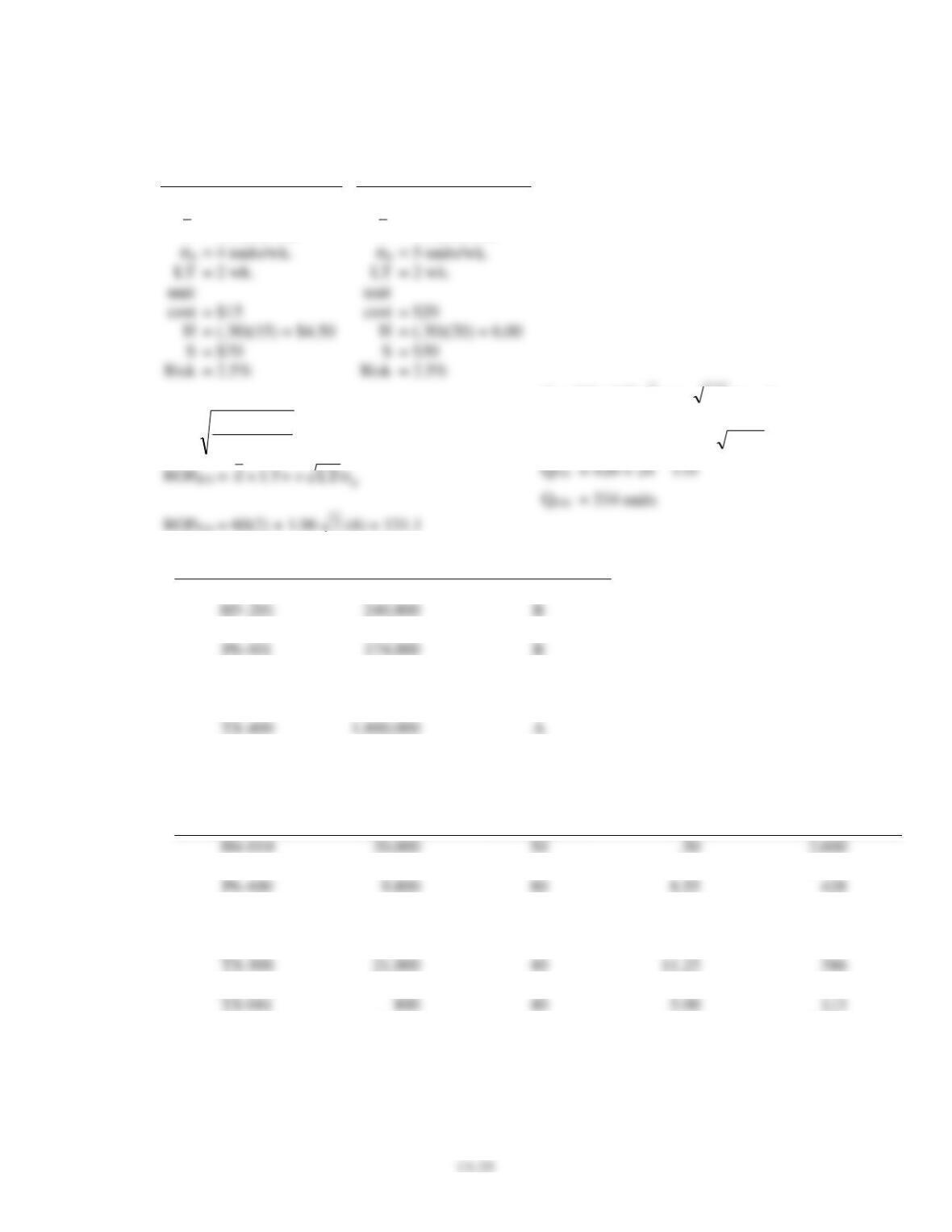
33. a.
Item
Annual $ volume
Classification
H4-010
50,000
C
240,800
B
P6-400
279,300
B
P6-401
174,000
B
P7-100
56,250
C
P9-103
165,000
C
TS-300
945,000
A
A
TS-041
16,000
C
V1-001
132,400
C
b.
Item
Estimated annual
demand
Ordering cost
Unit holding cost
($)
EOQ
20,000
.50
2,000
H5-201
60,200
60
.80
3,005
P6-400
9,800
8.55
428
P6-401
14,500
50
3.60
635
P7-100
6,250
50
2.70
481
P9-103
7,500
50
8.80
292
21,000
40
11.25
386
TS-400
45,000
40
10.00
600
800
40
5.00
113
V1-001
33,100
25
1.40
1,087
Chapter 13 – Inventory Management
13-26
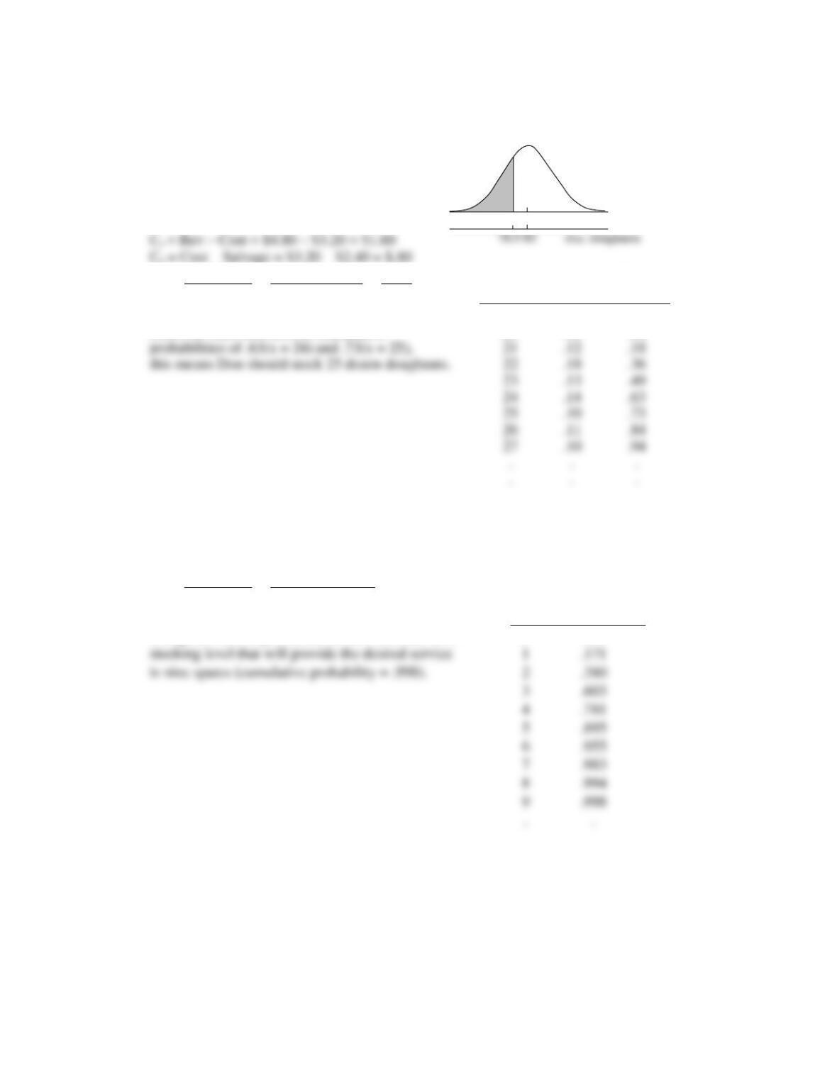
34.
SL =
Cs
=
$1.60
=
1.6
= .67
x
Cum.
Cs + Ce
$1.60 + $.80
2.4
Demand
P(x)
P(x)
19
.01
.01
Since this falls between the cumulative
20
.05
.06
probabilities of .63(x = 24) and .73(x = 25),
21
.12
.18
this means Don should stock 25 dozen doughnuts.
22
.18
.36
23
.13
.49
24
.14
.63
25
.10
.73
26
.11
.84
27
.10
.94
.
.
.
.
.
.
.
.
.
35.
Cs = $88,000
Ce = $100 + 1.45($100) = $245
a.
SL =
Cs
=
$88,000
= .9972
Cs + Ce
$88,000 + $245
[From Poisson Table with = 3.2]
x
Cum. Prob.
Using the Poisson probabilities, the minimum level
0
.041
stocking level that will provide the desired service
1
.171
is nine spares (cumulative probability = .998).
2
.380
3
.603
4
.781
5
.895
6
.955
7
.983
8
.994
9
.998
.
.
.
.
.
.
–.11 0 z-scale
.4545
Chapter 13 – Inventory Management
13-27
b.
47.10$C
C045.10C041.
s
s
ss
ss
=
=+
Carrying no spare parts is the best strategy if the shortage cost is less than or equal to $10.47
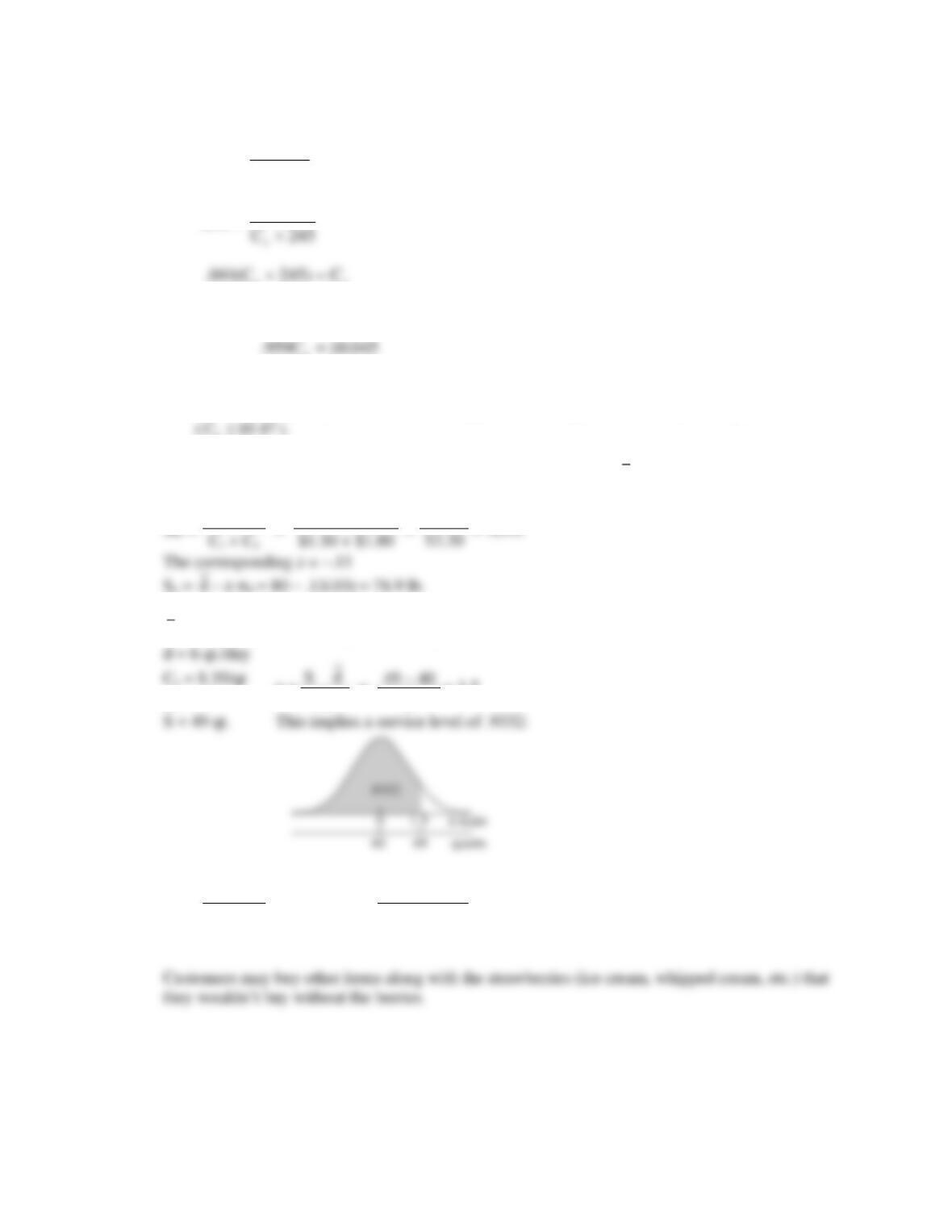
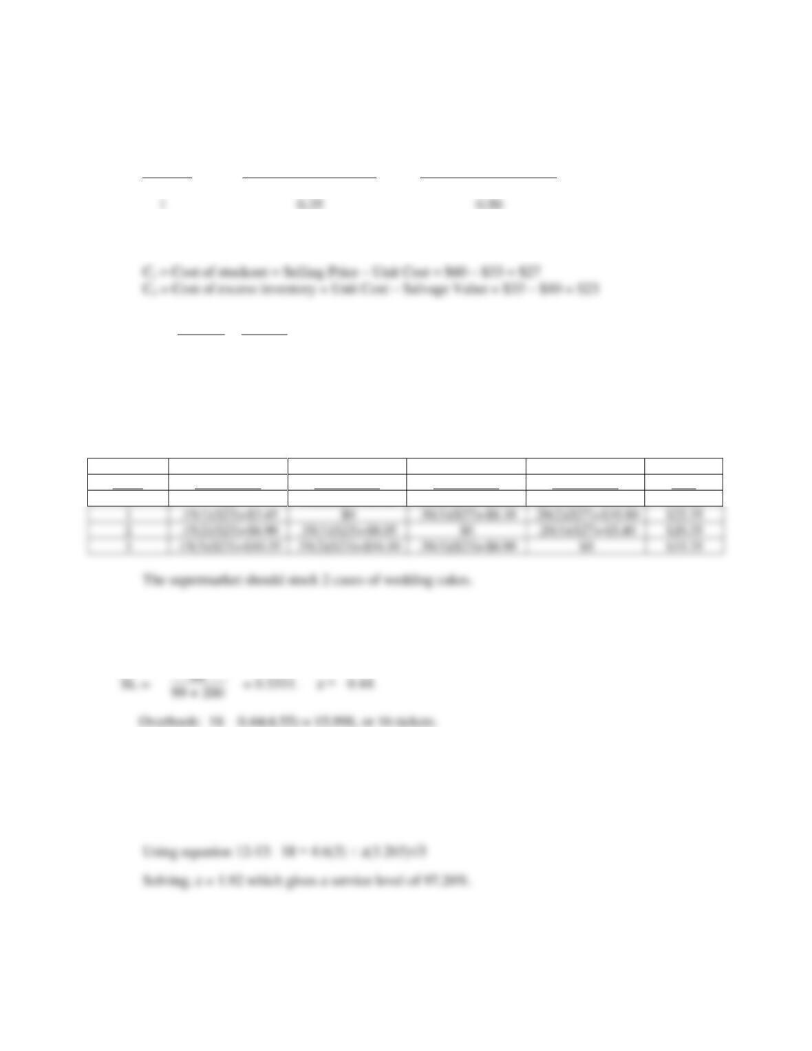
36.
Cs = Rev – Cost = $5.70 – $4.20 = $1.50/unit
d
= 80 lb./day
Ce = Cost – Salvage = $4.20 – $2.40 = $1.80/unit
d= 10 lb./day
SL =
= .4545
$3.30
Cs
$1.50
$1.50
37.
d
= 40 qt./day
A stocking level of 49 quarts translates into a z of + 1.5:
d = 6 qt./day
d
z =
=
= 1.5
Cs = ?
d
6
S = 49 qt.
This implies a service level of .9332:
SL =
Cs
Thus, .9332 =
Cs
Cs + Ce
Cs+ $.35
Solving for Cs we find: .9332(Cs + .35) = Cs; Cs = $4.89/qt.
C
041.
CC
C
SL
s
es
s
=
+
=
Chapter 13 – Inventory Management
13-28
38.
Cs = Rev – Cost = $12 – $9 = $3.00/cake
SL =
Cs
=
$3.00
= .40
Demand
Cum. Prob.
Cs + Ce
$3.00 + $4.50
0
.003
probability for demand of 4 and 5, the
2
.062
4
.285
6
.606
.
.
.
.
.
.
39.
Cs = $.10/burger x 4 burgers/lb. = $.40/lb.
Ce = Cost – Salvage = $1.00 – $.80 = $.20/lb.
Cs
The appropriate z is +.43.
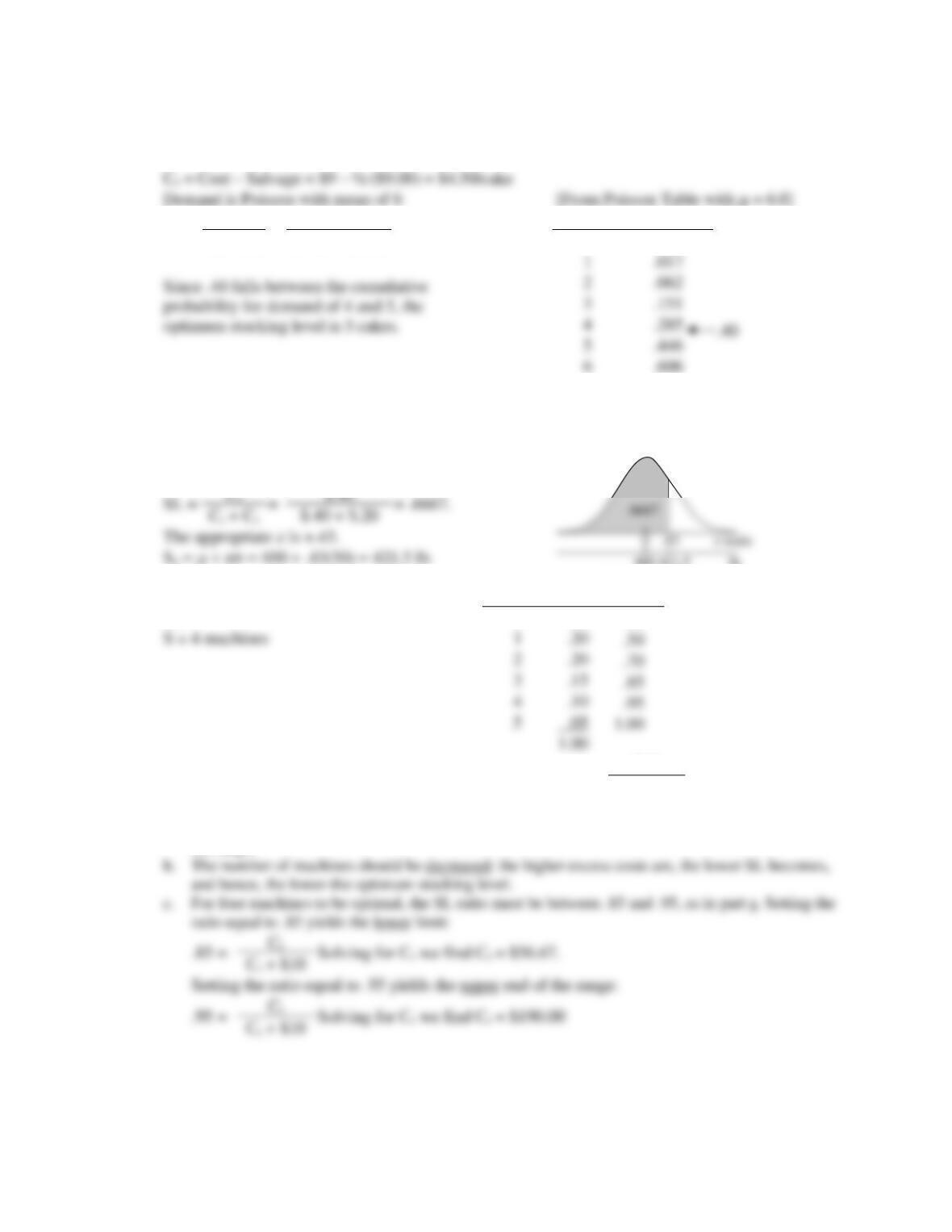
40.
Cs = $10/machine
Demand
Freq.
Cum.
Freq.
Ce = ?
0
.30
.30
S = 4 machines
2
.20
.70
4
.10
.95
a.
For four machines to be optimal, the SL ratio must be .85
$10
.95.
$10 + Ce
Setting the ratio equal to .85 and solving for Ce yields $1.76, which is the upper end of the range.
Setting the ratio equal to .95 and again solving for Ce , we find Ce = $.53, which is the lower end of
the range.
The number of machines should be decreased: the higher excess costs are, the lower SL becomes,
and hence, the lower the optimum stocking level.
ratio equal to .85 yields the lower limit:
Setting the ratio equal to .95 yields the upper end of the range:
.95 =
Solving for Cs we find Cs = $190.00
400 421.5 lb.
Demand is Poisson with mean of 6
Chapter 13 – Inventory Management
13-29
41. a. Ratio Method
# of spares Probability of Demand Cumulative Probability
1 0.50 0.60
3 0.15 1.00
Cs = Cost of stockout = ($500 per day) (2 days) = $1000
Ce = Cost of excess inventory = Unit cost – Salvage Value = $200 – $50 = $150
b. Tabular Method
Stocking
Demand = 0
Demand = 1
Demand = 2
Demand = 3
Expected
Level
Prob. = 0.10
Prob. = 0.50
Prob. = 0.25
Prob. = 0.15
Cost
0
$0
.50(1)($1000)=$500
.25(2)($1000)=$500
.15(3)($1000)=$450
$1,450
1
.10(1)($150)=$15
.25(1)($1000)=$250
2
.10(2)($150)=$30
.50(1)($150)=$75
.15(1)($1000)=$150
3
.10(3)($150)=$45
.25(1)($150)=$37.50
Chapter 13 – Inventory Management
13-30
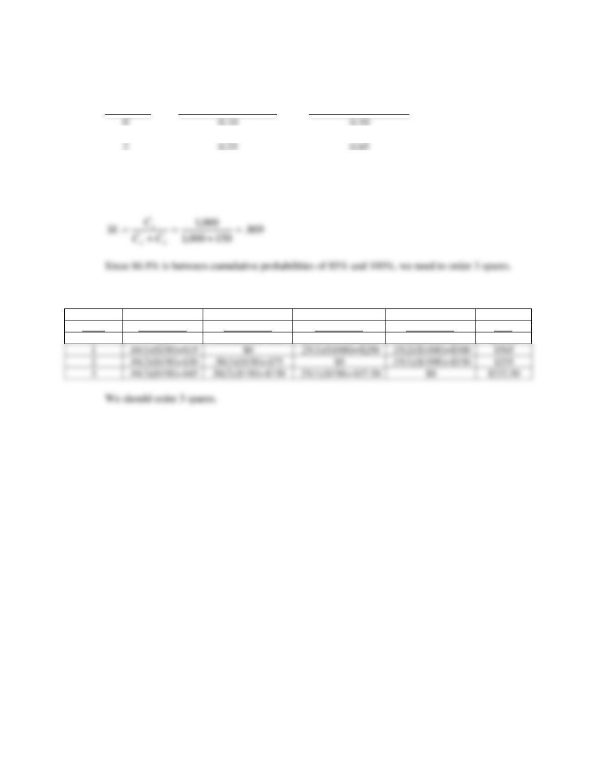
42. a. Ratio Method: Demand and the probabilities for the cases of wedding cakes are given in the
following table.
Demand Probability of Demand Cumulative Probability
0 0.15 0.15
2 0.30 0.80
3 0.20 1.00
54.
2327
27 =
+
=
+
=
es
s
CC
C
SL
Since the service level of 54% falls between cumulative probabilities of 50% and 80%, the
supermarket should stock 2 cases of wedding cakes.
b. Tabular Method
Stocking
Demand = 0
Demand = 1
Demand = 2
Demand = 3
Expected
Level
Prob. = 0.15
Prob. = 0.35
Prob. = 0.30
Prob. = 0.20
Cost
0
$0
.35(1)($27)=$9.45
.30(2)($27)=$16.20
.20(3)($27)=$16.20
$41.85
1
$0
.20(2)($27)=$10.80
$22.35
2
.35(1)($23)=$8.05
$0
.20(1)($27)=$5.40
$20.35
3
$0
$33.35
43. Cs = $99, Ce = $200
44. Mean usage = 4.6 units/day
Standard dev. = 1.265 units/day
LT = 3 days
ROP = 18
Chapter 13 – Inventory Management
13-31
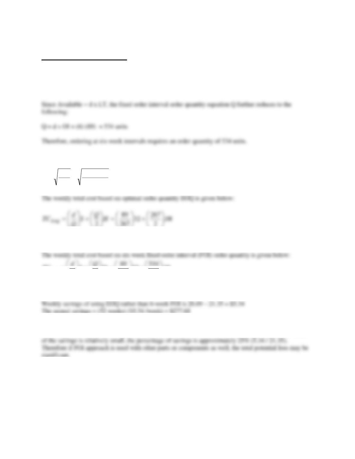
Case: UPD Manufacturing
1 Students must recognize that without demand variability, the fixed order interval order quantity
equation reduces to:
Q = d(LT + OI) – Available (because there is no safety stock)
On the other hand, the optimal order quantity is determined by using the basic EOQ equation.
267
08.
)32)(89(2
2=== h
dS
Q
weekTC
EOQ
/35.2168.1067.10
=+=
weekTC
H
S
Q
TC
FOI
FOI
/69.2636.2133.5
08.
2
32
534
2
=+=
+
=
+
=
2. The total annual savings as a result of switching from six-week FOI to EOQ are relatively small and
switching to the optimal order quantity may not be warranted. However, even though the absolute value
Chapter 13 – Inventory Management
13-32
Case: Harvey Industries
In order to improve the current inventory control system, the new president may want to consider the
following:
2. Currently, no paper work is used when items are withdrawn from the stockroom when they are
needed on the shop floor. Harvey Industries may either want to establish a procedure for
3. It appears that utilization of ABC inventory classification system is needed. The company
should never experience stockouts in their basic “C” items. ABC analysis will allow Harvey
Industries to establish an appropriate degree of control over items in terms of order quantity and
ordering frequency.
Case: Grill Rite
The president’s stance on steady output conflicts with seasonal demand. However, it is unlikely that this
will change. One alternative might be to identify a complementary product that would offset seasonal
demand for electric grills.