Chapter 13 – Problems 1-10 Note: This worksheet displays results only, you must copy the shaded
<Back area into the corresponding template to make additional calculations.
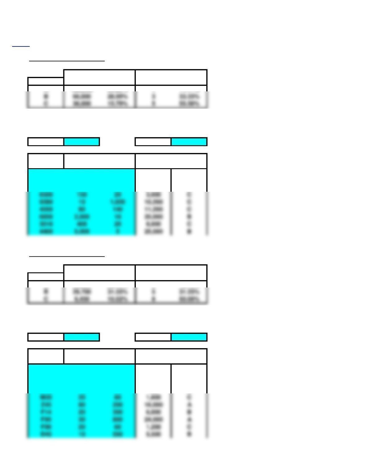
1. ABC Classification System
Dollar Amount Number of Items
Class Total Percent Total Percent
A126,000 55.26% 111.11%
Enter lower limit for dollar amount:
A126,000 B20,000
Unit Dollar
Item Usage Cost Amount Class
4021 90 1,400 126,000 A
9402 300 12 3,600 C
4066 30 700 21,000 B
6500 150 20 3,000 C
4050 80 140 11,200 C
3010 400 20 8,000 C
2. ABC Classification System
Dollar Amount Number of Items
Class Total Percent Total Percent
A55,000 58.43% 318.75%
Enter lower limit for dollar amount:
A15,000 B4,800
Unit Dollar
Item Usage Cost Amount Class
K34 10 200 2,000 C
K35 25 600 15,000 A
K36 36 150 5,400 B
M10 16 25 400 C
M20 20 80 1,600 C
D45 10 550 5,500 B
D48 12 90 1,080 C
D52 15 110 1,650 C
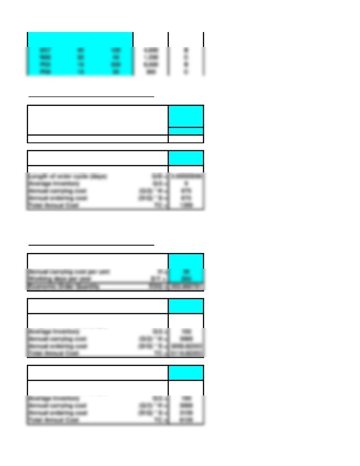
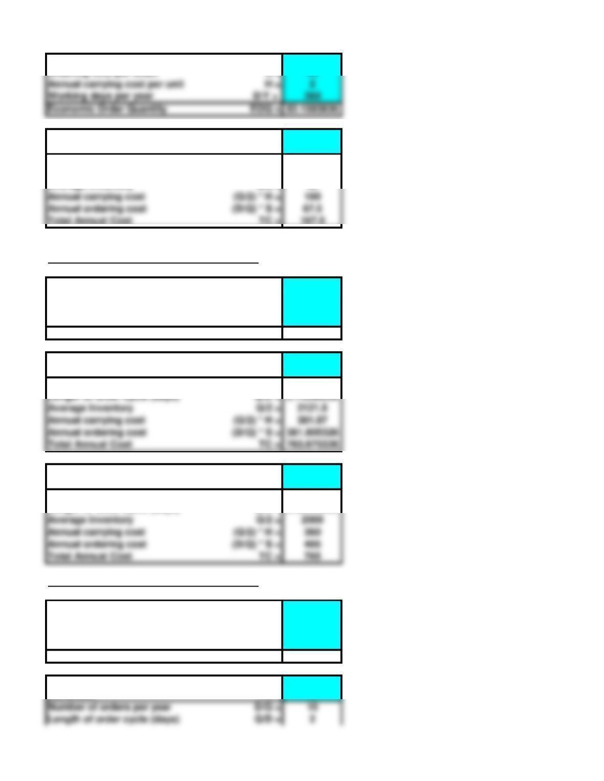
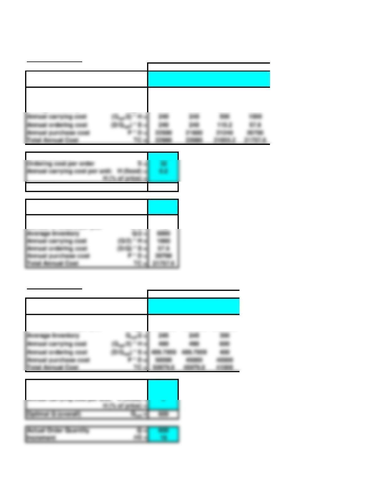
3. Basic Economic Order Quantity (EOQ) Model
Annual Demand D = 1215
Ordering cost per order S = 10
Annual carrying cost per unit H = 75
Working days per year D/Y = 240
Economic Order Quantity EOQ = 18
Actual Order Quantity Q = 18
Increment DQ = 10
Number of orders per year D/Q = 67.5
Length of order cycle (days) Q/D = 3.55555556
Average Inventory Q/2 = 9
Annual carrying cost (Q/2) * H = 675
Annual ordering cost (D/Q) * S = 675
Total Annual Cost TC = 1350
For part d, if Q remains at 18 then TAC goes up by 81,
if Q is decreased to 17 (new EOQ) then TAC goes up by 78.71.
4. Basic Economic Order Quantity (EOQ) Model
Annual Demand D = 10400
Ordering cost per order S = 60
Annual carrying cost per unit H = 30
Working days per year D/Y = 260
Economic Order Quantity EOQ = 203.960781
Actual Order Quantity Q = 204
Increment DQ = 1
Number of orders per year D/Q = 50.9803922
Length of order cycle (days) Q/D = 5.1
Average Inventory Q/2 = 102
Annual ordering cost (D/Q) * S = 3058.82353
Total Annual Cost TC = 6118.82353
4d. Actual Order Quantity Q = 200
Increment DQ = 1
Number of orders per year D/Q = 52
Length of order cycle (days) Q/D = 5
Average Inventory Q/2 = 100
Annual carrying cost (Q/2) * H = 3000
Annual ordering cost (D/Q) * S = 3120
D57 40 120 4,800 B
N08 30 40 1,200 C
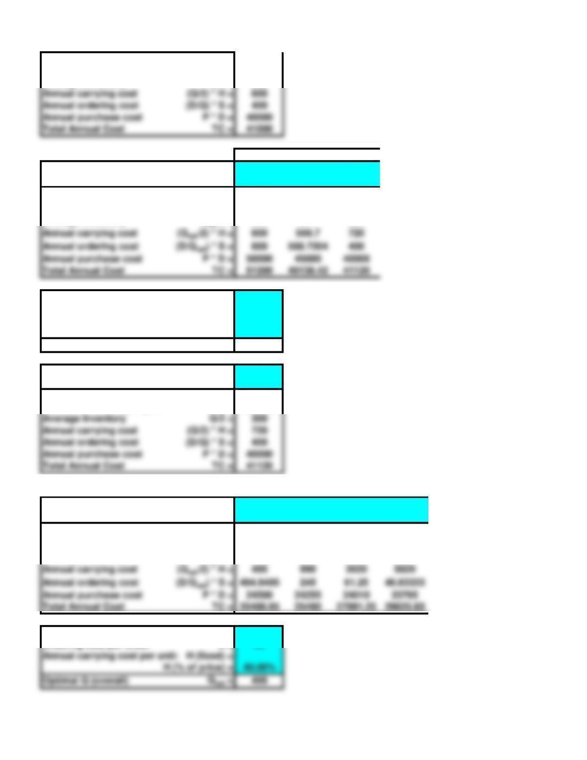
5. Basic Economic Order Quantity (EOQ) Model
Annual Demand D = 9000
Ordering cost per order S = 20
Actual Order Quantity Q = 775
Increment DQ = 1
Number of orders per year D/Q = 11.6129032
Length of order cycle (days) Q/D = 22.3888889
Average Inventory Q/2 = 387.5
Annual carrying cost (Q/2) * H = 232.5
Annual ordering cost (D/Q) * S = 232.258065
Total Annual Cost TC = 464.758065
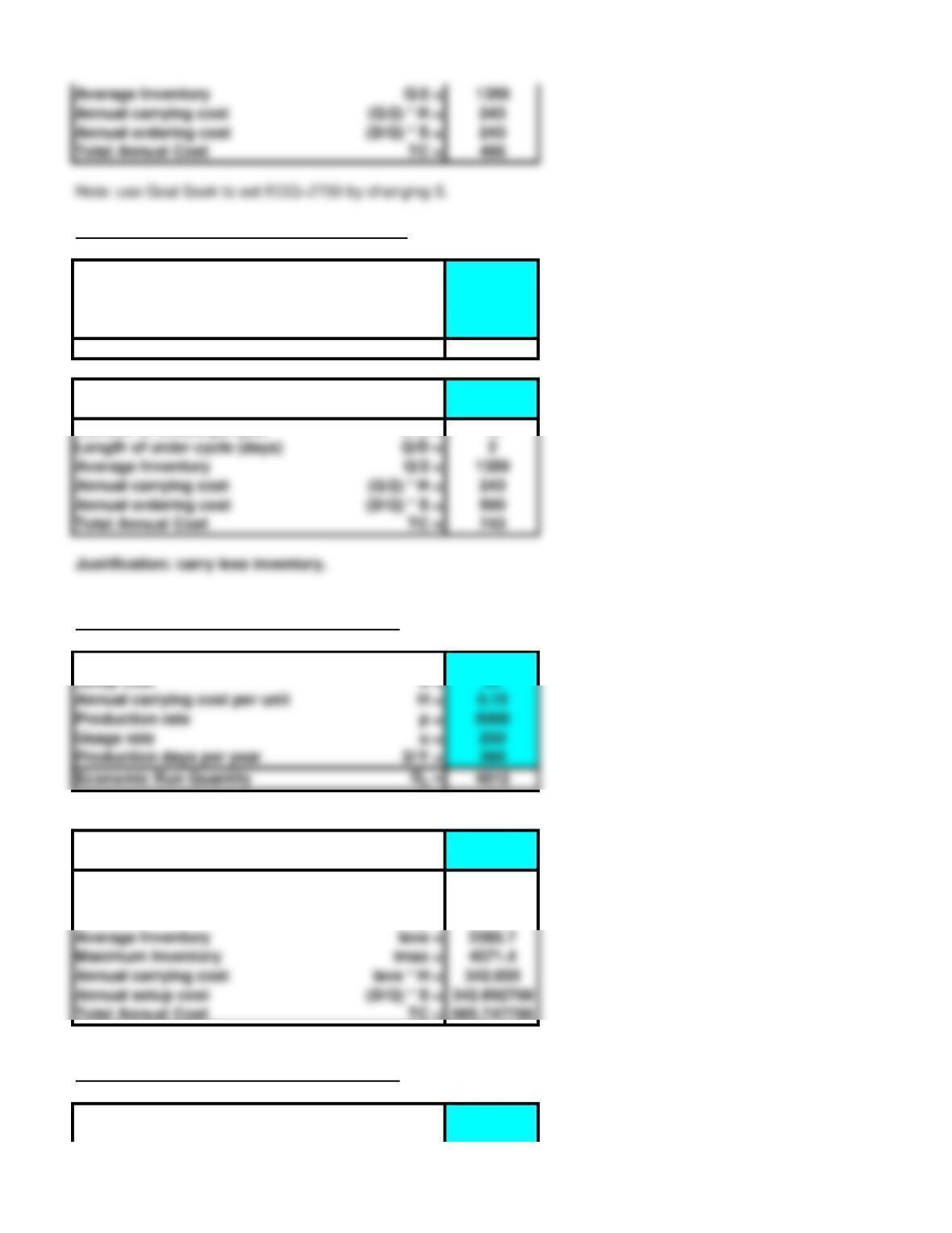
Actual Order Quantity Q = 1500
Increment DQ = 1
Number of orders per year D/Q = 6
Length of order cycle (days) Q/D = 43.3333333
Average Inventory Q/2 = 750
Annual carrying cost (Q/2) * H = 450
Annual ordering cost (D/Q) * S = 120
Total Annual Cost TC = 570
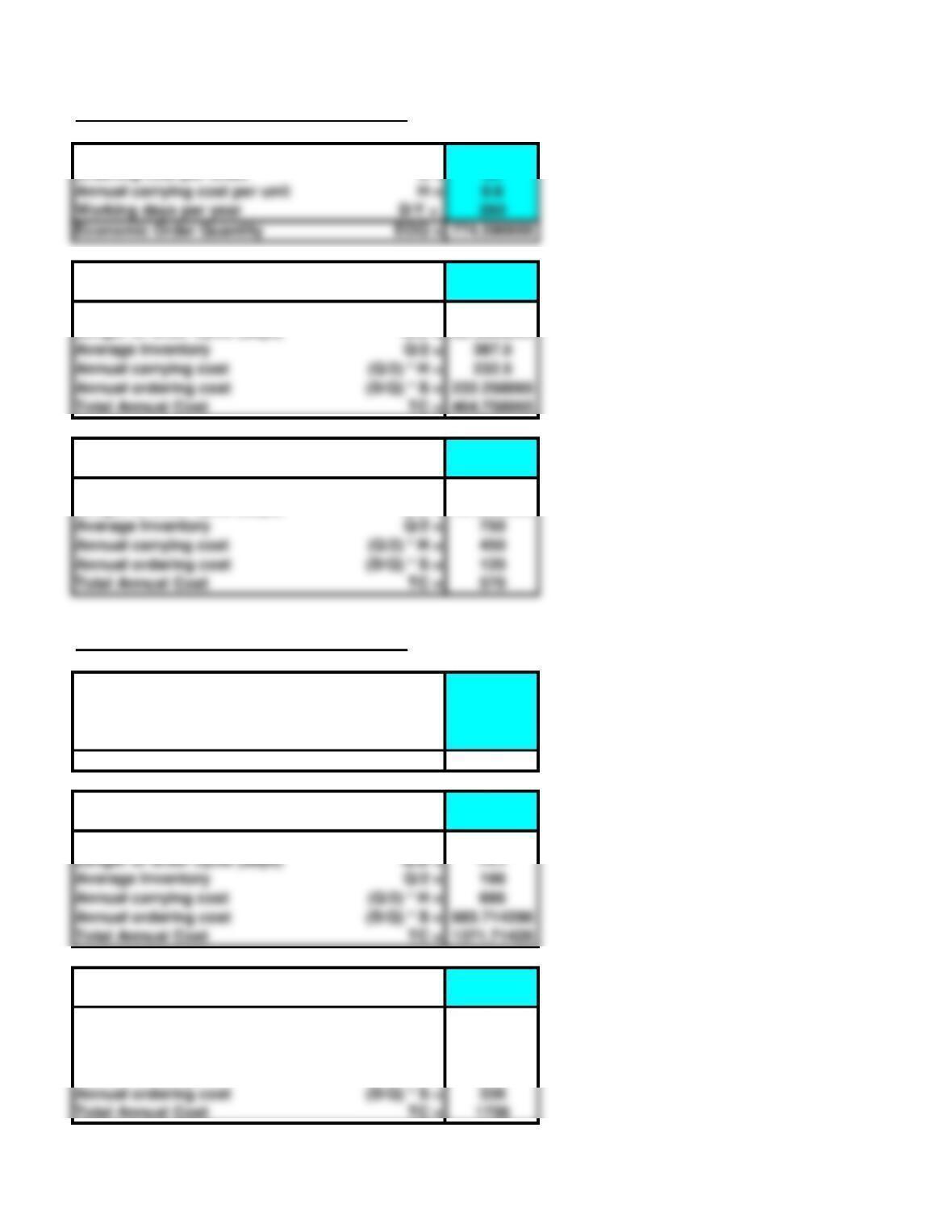
6. Basic Economic Order Quantity (EOQ) Model
Annual Demand D = 9600
Ordering cost per order S = 28
Annual carrying cost per unit H = 3.5
Working days per year D/Y = 360
Economic Order Quantity EOQ = 391.918359
Actual Order Quantity Q = 392
Increment DQ = 1
Number of orders per year D/Q = 24.4897959
Length of order cycle (days) Q/D = 14.7
Average Inventory Q/2 = 196
Annual carrying cost (Q/2) * H = 686
Annual ordering cost (D/Q) * S = 685.714286
Total Annual Cost TC = 1371.71429
Actual Order Quantity Q = 800
Increment DQ = 1
Number of orders per year D/Q = 12
Length of order cycle (days) Q/D = 30
Average Inventory Q/2 = 400
Annual carrying cost (Q/2) * H = 1400
Annual ordering cost (D/Q) * S = 336
Annual carrying cost per unit H = 0.6
Working days per year D/Y = 260
Economic Order Quantity EOQ = 774.596669
7a. Basic Economic Order Quantity (EOQ) Model
Annual Demand D = 100
Ordering cost per order S = 55
Actual Order Quantity Q = 75
Increment DQ = 1
Number of orders per year D/Q = 1.33333333
Length of order cycle (days) Q/D = 270
Average Inventory Q/2 = 37.5
Annual carrying cost (Q/2) * H = 75
Annual ordering cost (D/Q) * S = 73.3333333
Basic Economic Order Quantity (EOQ) Model
Annual Demand D = 150
Ordering cost per order S = 55
Annual carrying cost per unit H = 2
Actual Order Quantity Q = 91
Increment DQ = 1
Number of orders per year D/Q = 1.64835165
Length of order cycle (days) Q/D = 218.4
Average Inventory Q/2 = 45.5
Annual carrying cost (Q/2) * H = 91
Annual ordering cost (D/Q) * S = 90.6593407
7c. Basic Economic Order Quantity (EOQ) Model
Annual Demand D = 100
Ordering cost per order S = 45
Annual carrying cost per unit H = 2
Actual Order Quantity Q = 50
Increment DQ = 1
Number of orders per year D/Q = 2
Length of order cycle (days) Q/D = 180
Average Inventory Q/2 = 25
Annual carrying cost (Q/2) * H = 50
Annual ordering cost (D/Q) * S = 90
Basic Economic Order Quantity (EOQ) Model
Annual carrying cost per unit H = 2
Annual Demand D = 150
Ordering cost per order S = 45
Actual Order Quantity Q = 100
Increment DQ = 1
Number of orders per year D/Q = 1.5
Length of order cycle (days) Q/D = 240
Average Inventory Q/2 = 50
Annual carrying cost (Q/2) * H = 100
Annual ordering cost (D/Q) * S = 67.5
Total Annual Cost TC = 167.5
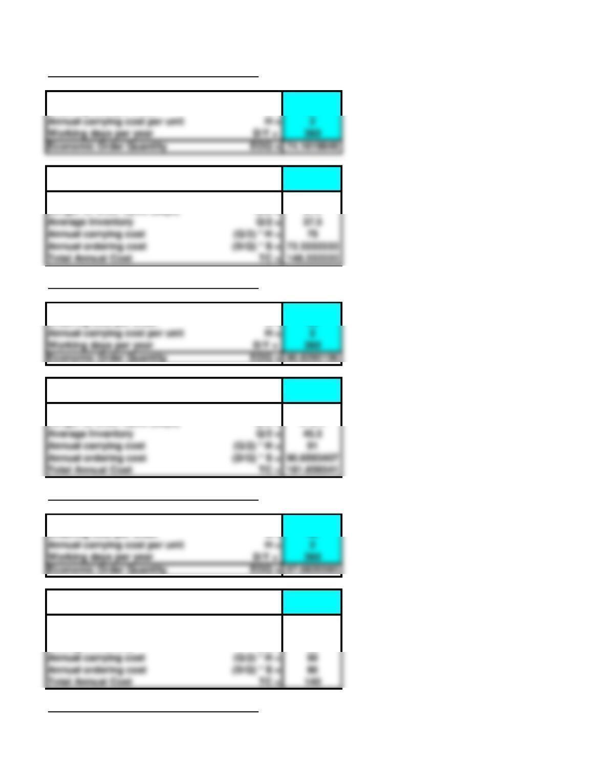
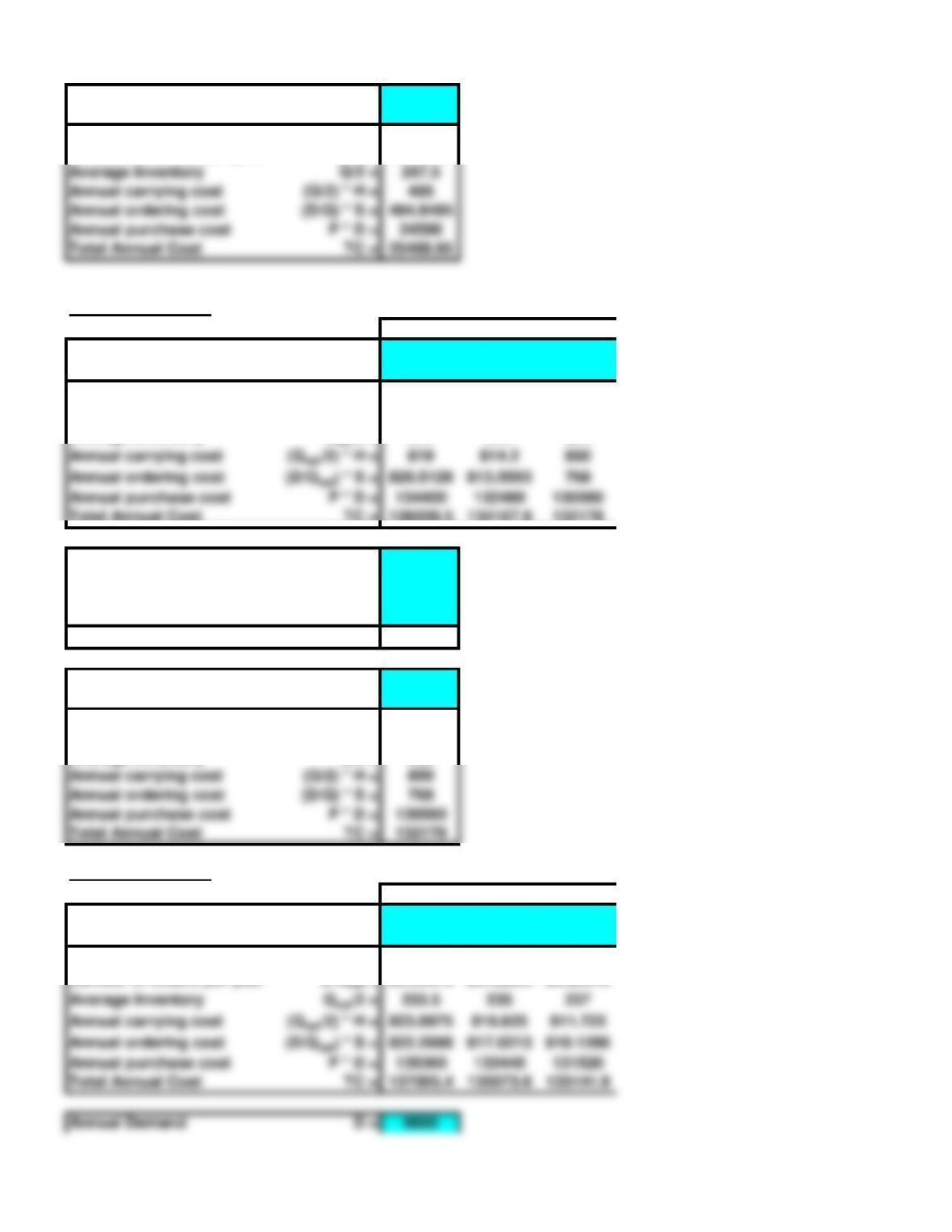
8a. Basic Economic Order Quantity (EOQ) Model
Annual Demand D = 27000
Ordering cost per order S = 60
Annual carrying cost per unit H = 0.18
Working days per year D/Y = 20
Economic Order Quantity EOQ = 4242.64069
Actual Order Quantity Q = 4243
Increment DQ = 1
Number of orders per year D/Q = 6.36342211
Length of order cycle (days) Q/D = 3.14296296
Average Inventory Q/2 = 2121.5
Annual carrying cost (Q/2) * H = 381.87
Annual ordering cost (D/Q) * S = 381.805326
Total Annual Cost TC = 763.675326
Actual Order Quantity Q = 4000
Increment DQ = 1
Number of orders per year D/Q = 6.75
Length of order cycle (days) Q/D = 2.96296296
Average Inventory Q/2 = 2000
Annual carrying cost (Q/2) * H = 360
Annual ordering cost (D/Q) * S = 405
Total Annual Cost TC = 765
8b. Basic Economic Order Quantity (EOQ) Model
Annual Demand D = 27000
Ordering cost per order S = 24.3
Annual carrying cost per unit H = 0.18
Working days per year D/Y = 20
Economic Order Quantity EOQ = 2700
Actual Order Quantity Q = 2700
Increment DQ = 1
Number of orders per year D/Q = 10
Length of order cycle (days) Q/D = 2
Annual carrying cost per unit H = 2
Working days per year D/Y = 360
Economic Order Quantity EOQ = 82.1583836
8c. Basic Economic Order Quantity (EOQ) Model
Annual Demand D = 27000
Ordering cost per order S = 50
Annual carrying cost per unit H = 0.18
Working days per year D/Y = 20
Economic Order Quantity EOQ = 3872.98335
Actual Order Quantity Q = 2700
Increment DQ = 1
Number of orders per year D/Q = 10
Length of order cycle (days) Q/D = 2
Average Inventory Q/2 = 1350
Annual carrying cost (Q/2) * H = 243
Annual ordering cost (D/Q) * S = 500
Total Annual Cost TC = 743
Justification: carry less inventory.
9. Economic Production Quantity (EPQ) Model
Annual Demand D = 75000
Setup cost S = 22
Annual carrying cost per unit H = 0.15
Production rate p = 5000
Usage rate u = 250
Production days per year D/Y = 300
Actual Run Quantity Q = 4812
Increment DQ = 100
Number of runs per year D/Q = 15.5860349
Cycle time Q/u = 19.248
Run time Q/p = 0.9624
Average Inventory Iave = 2285.7
Maximum Inventory Imax = 4571.4
Annual carrying cost Iave * H = 342.855
Annual setup cost (D/Q) * S = 342.892768
Total Annual Cost TC = 685.747768
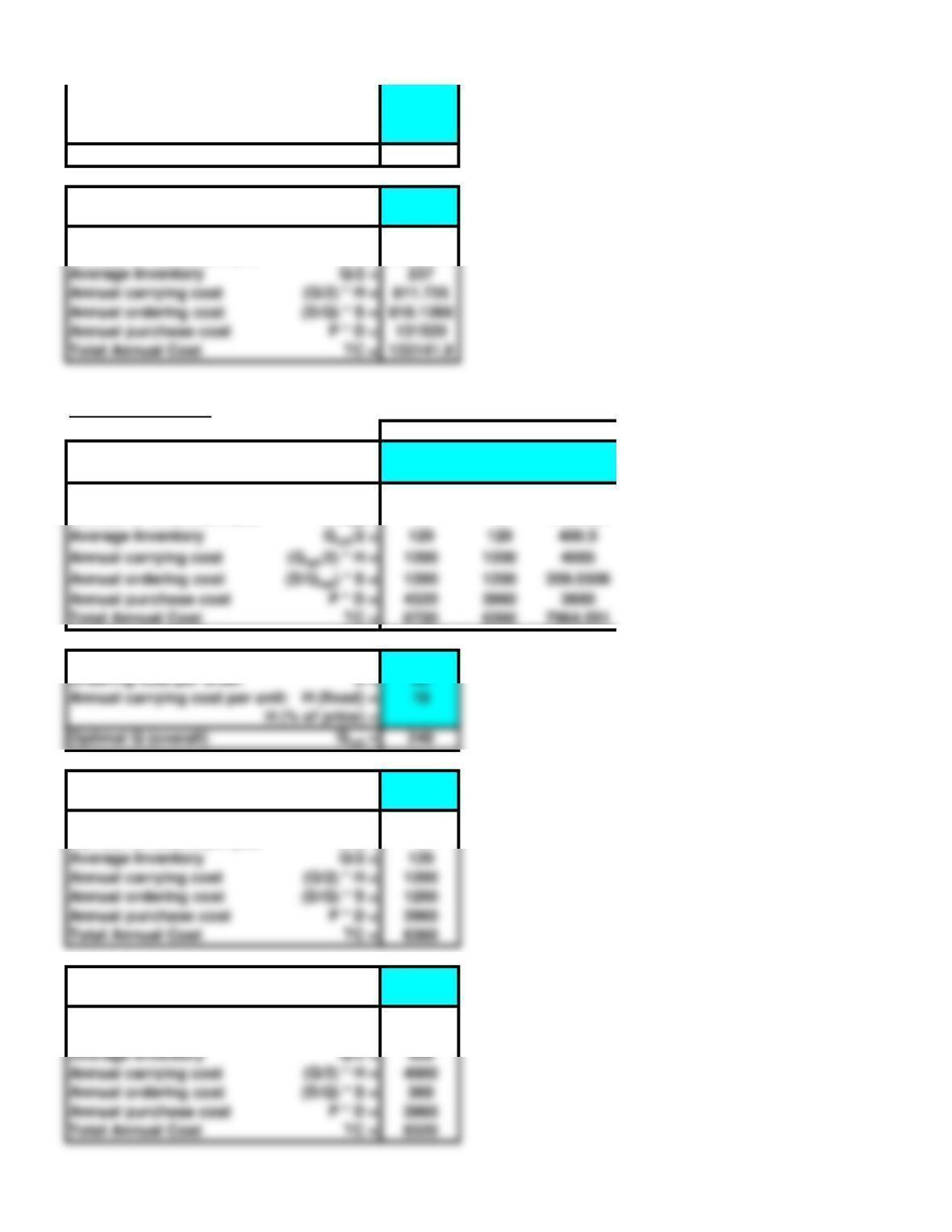
10. Economic Production Quantity (EPQ) Model
Annual Demand D = 80000
Setup cost S = 100
Average Inventory Q/2 = 1350
Annual ordering cost (D/Q) * S = 243
Total Annual Cost TC = 486
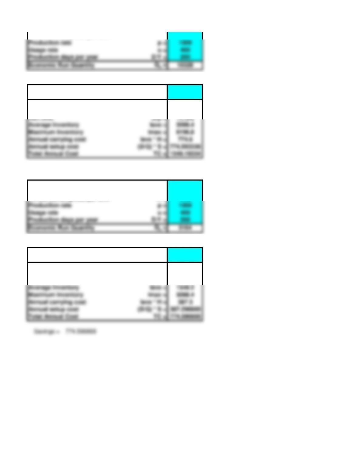
Annual carrying cost per unit H = 0.25
Actual Run Quantity Q = 10328
Increment DQ = 100
Number of runs per year D/Q = 7.74593338
Cycle time Q/u = 25.82
Run time Q/p = 10.328
Average Inventory Iave = 3098.4
Maximum Inventory Imax = 6196.8
Annual carrying cost Iave * H = 774.6
Annual setup cost (D/Q) * S = 774.593338
Note: D, H, p, and u have been expressed in bags, not tons.
10e. Annual Demand D = 80000
Setup cost S = 25
Annual carrying cost per unit H = 0.25
Production rate p = 1000
Usage rate u = 400
Actual Run Quantity Q = 5164
Increment DQ = 100
Number of runs per year D/Q = 15.4918668
Cycle time Q/u = 12.91
Run time Q/p = 5.164
Average Inventory Iave = 1549.2
Maximum Inventory Imax = 3098.4
Annual carrying cost Iave * H = 387.3
Annual setup cost (D/Q) * S = 387.296669
Usage rate u = 400
Chapter 13 – Problems 11-20 Note: This worksheet displays results only, you must copy the shaded
<Back area into the corresponding template to make additional calculations.
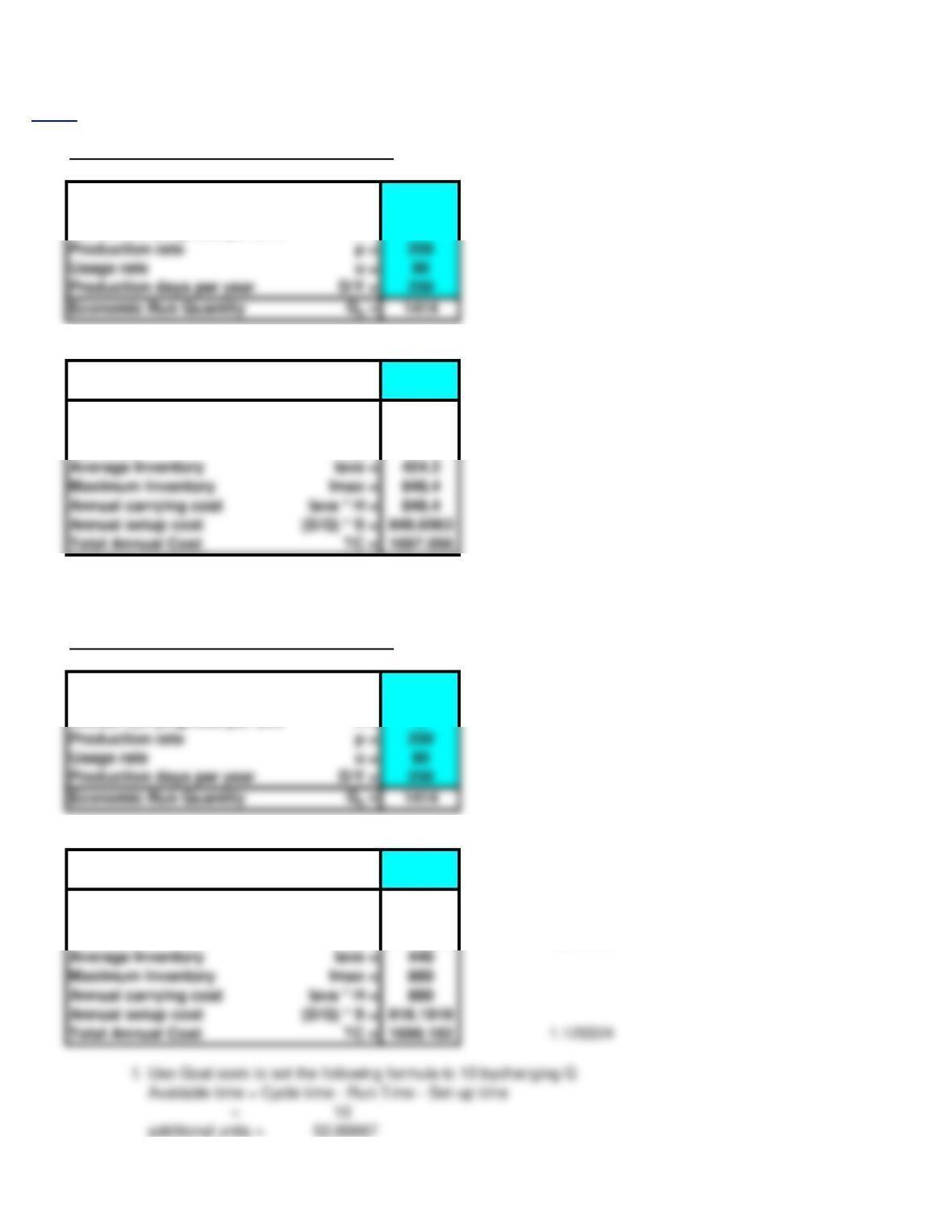
11. Economic Production Quantity (EPQ) Model
Annual Demand D = 20000
Setup cost S = 60
Annual carrying cost per unit H = 2
Actual Run Quantity Q = 1414
Increment FALSE DQ = 100
Number of runs per year D/Q = 14.14427
Cycle time Q/u = 17.675
Run time Q/p = 7.07
Average Inventory Iave = 424.2
Maximum Inventory Imax = 848.4
Annual carrying cost
Annual setup cost (D/Q) * S = 848.6563
c. p – u = 120
d. Cycle time – Run Time – 1 = 9.605
11f. Economic Production Quantity (EPQ) Model
Annual Demand D = 20000
Setup cost S = 60
Annual carrying cost per unit H = 2
Production rate p = 200
Usage rate u = 80
Actual Run Quantity Q = 1466.667 52.66667
Increment DQ = 100
Number of runs per year D/Q = 13.63636
Cycle time Q/u = 18.33333 0.658333
Run time Q/p = 7.333333 0.263333
Average Inventory Iave = 440
Maximum Inventory Imax = 880
Annual carrying cost
Annual setup cost (D/Q) * S = 818.1818
Production rate p = 200
Usage rate u = 80
additional cost = 1.125524
13. Quantity Discounts
Price Level: 1 2 3 4
Minimum quantity for price
Qmin = 1000 2000 5000 10000
Price P = 1.25 1.20 1.18 1.15
Optimal Q (for each price)
Qopt = 2400 2400 5000 10000
Number of orders per year
D/Qopt = 7.5 7.5 3.6 1.8
Average Inventory
Qopt/2 = 1200 1200 2500 5000
Annual Demand D = 18000
Ordering cost per order S = 32
Annual carrying cost per unit: H (fixed) = 0.2
Optimal Q (overall)
Qopt = 10000
Actual Order Quantity Q = 10000
Increment DQ = 100
Price P = 1.15
Number of orders per year D/Q = 1.8
Annual ordering cost (D/Q) * S = 57.6
Annual purchase cost P * D = 20700
Total Annual Cost TC = 21757.6
14a. Quantity Discounts
Price Level: 1 2 3
Minimum quantity for price
Qmin = 1400 600
Price P = 10.00 9.00 8.00
Optimal Q (for each price)
Qopt = 490 490 600
Number of orders per year
D/Qopt = 10.20408 10.20408 8.333333
Qopt/2 = 245 245 300
Annual purchase cost P * D = 50000 45000 40000
Total Annual Cost TC = 50979.8 45979.8 41000
Annual Demand D = 5000
Ordering cost per order S = 48
Annual carrying cost per unit: H (fixed) = 2
Actual Order Quantity Q = 600
Annual purchase cost P * D = 22500 21600 21240 20700
Total Annual Cost TC = 22980 22080 21855.2 21757.6
Price P = 8
Number of orders per year D/Q = 8.333333
Average Inventory Q/2 = 300
Price Level: 1 2 3
14b. Minimum quantity for price
Qmin = 1400 600
Price P = 10.00 9.00 8.00
Optimal Q (for each price)
Qopt = 400 422 600
Number of orders per year
D/Qopt = 12.5 11.84834 8.333333
Average Inventory
Qopt/2 = 200 211 300
Annual purchase cost P * D = 50000 45000 40000
Total Annual Cost TC = 51200 46138.42 41120
Annual Demand D = 5000
Ordering cost per order S = 48
Annual carrying cost per unit: H (fixed) =
2 FALSE H (% of price) = 30.00%
Optimal Q (overall)
Qopt = 600
Actual Order Quantity Q = 600
Increment DQ = 10
Price P = 8
Number of orders per year D/Q = 8.333333
Average Inventory Q/2 = 300
Annual ordering cost (D/Q) * S = 400
Annual purchase cost P * D = 40000
Total Annual Cost TC = 41120
15. Minimum quantity for price
Qmin = 11000 4000 6000
Price P = 5.00 4.95 4.90 4.85
Optimal Q (for each price)
Qopt = 495 1000 4000 6000
Number of orders per year
D/Qopt = 9.89899 4.9 1.225 0.816667
Average Inventory
Qopt/2 = 247.5 500 2000 3000
Annual purchase cost P * D = 24500 24255 24010 23765
Total Annual Cost TC = 25489.95 25490 27991.25 29625.83
Annual Demand D = 4900
Ordering cost per order S = 50
Annual carrying cost per unit: H (fixed) =
Annual ordering cost (D/Q) * S = 400
Annual purchase cost P * D = 40000
Total Annual Cost TC = 41000
Actual Order Quantity Q = 495
Increment DQ = 10
Price P = 5
Number of orders per year D/Q = 9.89899
16. Quantity Discounts
Price Level: 1 2 3
A Minimum quantity for price
Qmin = 1200 500
Price P = 14.00 13.80 13.60
Optimal Q (for each price)
Qopt = 468 472 500
Number of orders per year
D/Qopt = 20.51282 20.33898 19.2
Average Inventory
Qopt/2 = 234 236 250
Annual purchase cost P * D = 134400 132480 130560
Total Annual Cost TC = 136039.5 134107.8 132178
Annual Demand D = 9600
Ordering cost per order S = 40
Annual carrying cost per unit: H (fixed) =
2 FALSE H (% of price) = 25.00%
Optimal Q (overall)
Qopt = 500
Actual Order Quantity Q = 500
Increment DQ = 10
Price P = 13.6
Number of orders per year D/Q = 19.2
Average Inventory Q/2 = 250
Annual ordering cost (D/Q) * S = 768
Annual purchase cost P * D = 130560
Total Annual Cost TC = 132178
Quantity Discounts
Price Level: 1 2 3
B Minimum quantity for price
Qmin = 1150 350
Price P = 14.10 13.90 13.70
Optimal Q (for each price)
Qopt = 467 470 474
Number of orders per year
D/Qopt = 20.55675 20.42553 20.25316
Qopt/2 = 233.5 235 237
Annual purchase cost P * D = 135360 133440 131520
Annual Demand D = 9600
Annual ordering cost (D/Q) * S = 494.9495
Annual purchase cost P * D = 24500
Total Annual Cost TC = 25489.95
Ordering cost per order S = 40
Annual carrying cost per unit: H (fixed) =
2 FALSE H (% of price) = 25.00%
Optimal Q (overall)
Qopt = 474
Actual Order Quantity Q = 474
Increment DQ = 10
Price P = 13.7
Number of orders per year D/Q = 20.25316
17. Quantity Discounts
Price Level: 1 2 3
Minimum quantity for price
Qmin = 1200 801
Price P = 1.20 1.10 1.00
Optimal Q (for each price)
Qopt = 240 240 801
Number of orders per year
D/Qopt = 15 15 4.494382
Annual purchase cost P * D = 4320 3960 3600
Total Annual Cost TC = 6720 6360 7964.551
Annual Demand D = 3600
Ordering cost per order S = 80
Annual carrying cost per unit: H (fixed) = 10
Qopt = 240
Actual Order Quantity Q = 240
Increment DQ = 10
Price P = 1.1
Number of orders per year D/Q = 15
Annual purchase cost P * D = 3960
Total Annual Cost TC = 6360
Actual Order Quantity Q = 800
Increment DQ = 10
Price P = 1.1
Number of orders per year D/Q = 4.5
Annual ordering cost (D/Q) * S = 360
Annual purchase cost P * D = 3960
Annual ordering cost (D/Q) * S = 810.1266
Annual purchase cost P * D = 131520
Total Annual Cost TC = 133141.9
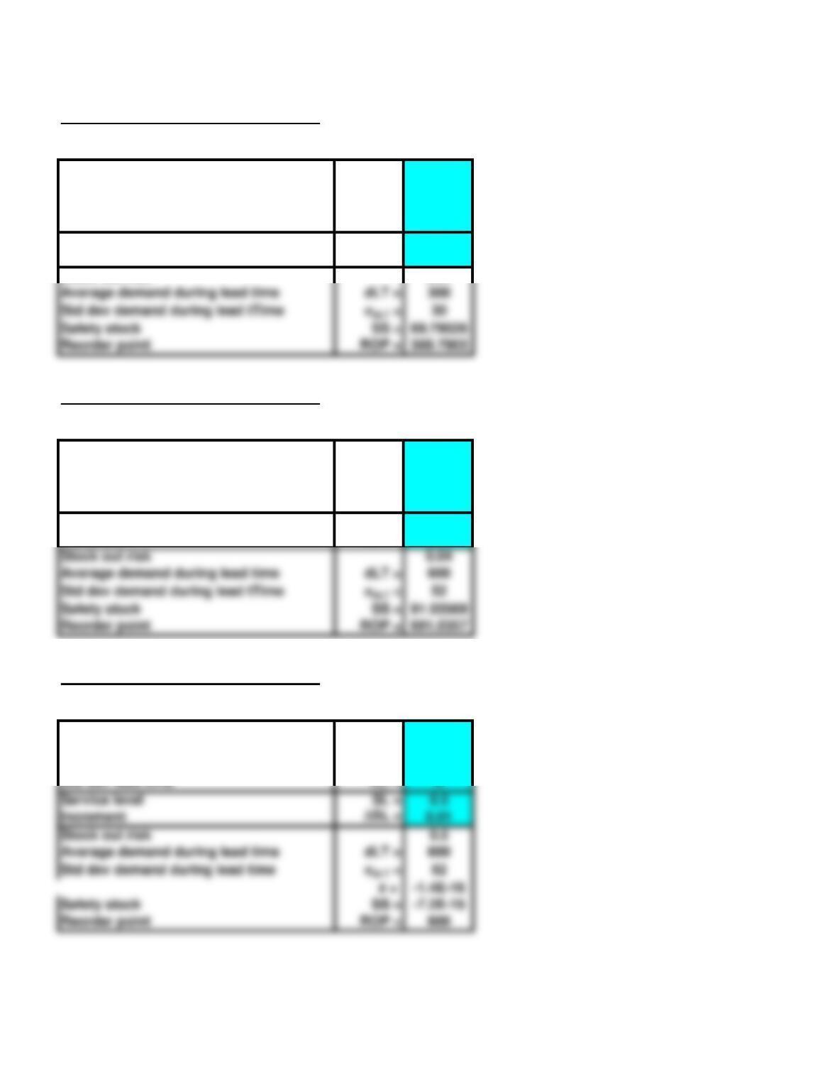
19. Reorder Point (ROP) with EOQ Ordering
Average demand d = 300
Std dev demand
sd = 30
Average lead time LT = 1
Std dev lead time
sLT = 0
Service level SL = 0.99
Increment DSL = 0.01
Stock out risk 0.01
20. Reorder Point (ROP) with EOQ Ordering
Average demand d = 600
Std dev demand
sd = 52
Average lead time LT = 1
Std dev lead time
sLT = 0
Service level SL = 0.96
Increment DSL = 0.01
Stock out risk 0.04
Average demand during lead time dLT = 600
Safety stock SS = 91.03569
20c. Reorder Point (ROP) with EOQ Ordering
Average demand d = 600
Std dev demand sd = 52
Average lead time LT = 1
Std dev lead time
sLT = 0
Service level SL = 0.5
Increment DSL = 0.01
Stock out risk 0.5
Average demand during lead time dLT = 600
Safety stock SS = -7.2E-15
Average demand during lead time dLT = 300
Chapter 13 – Problems 20-28 Note: This worksheet displays results only, you must copy the shaded
<Back area into the corresponding template to make additional calculations.
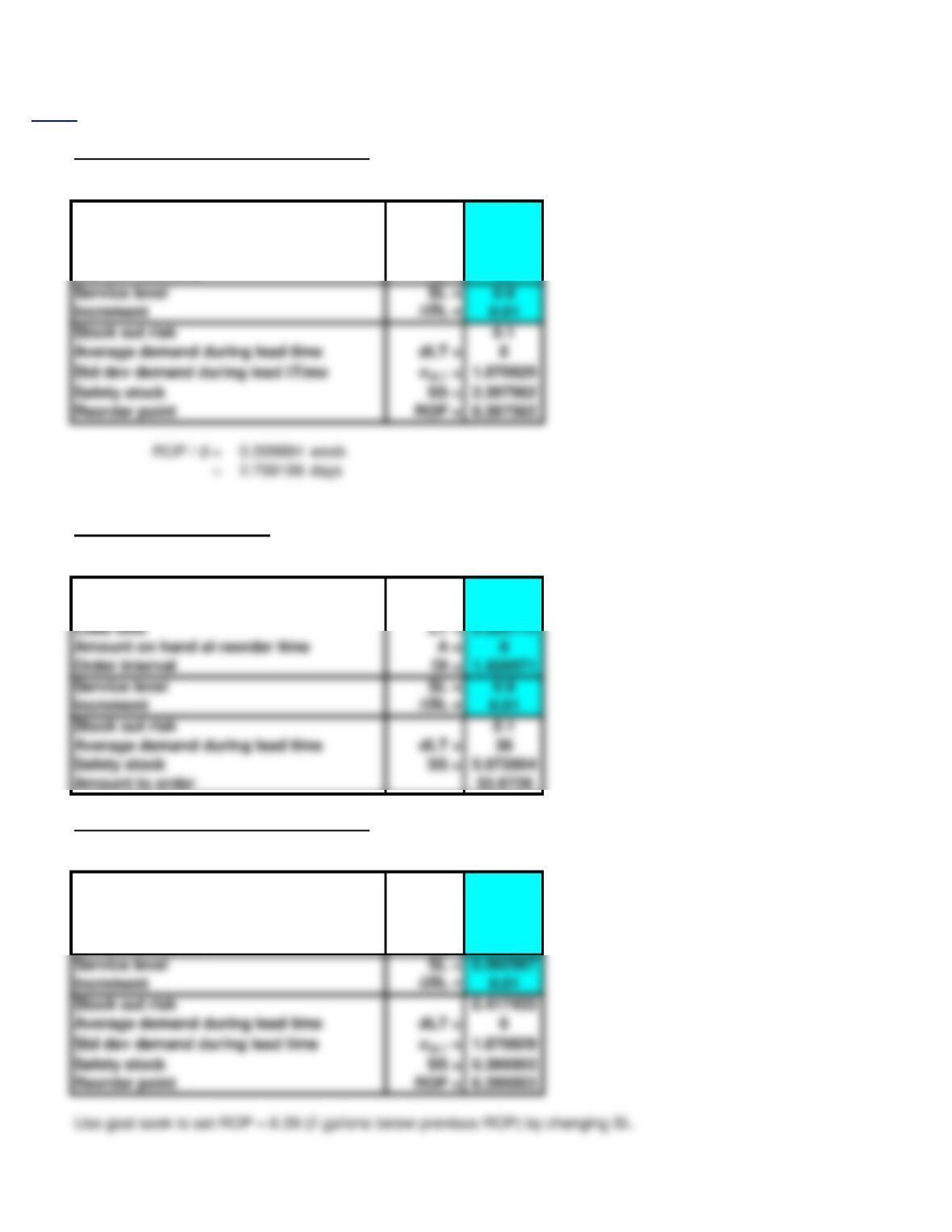
21a. Reorder Point (ROP) with EOQ Ordering
Average demand d = 21
Std dev demand
sd = 3.5
Average lead time LT = 0.285714
Std dev lead time
sLT = 0
21b. Fixed Order Interval Model
Average demand d = 21
Std dev demand
sd = 3.5
Lead time LT = 0.285714
Amount on hand at reorder time A = 8
Service level SL = 0.9
Stock out risk 0.1
Average demand during lead time dLT = 36
Safety stock SS = 5.872804
22c. Reorder Point (ROP) with EOQ Ordering
Average demand d = 21
Std dev demand
sd = 3.5
Average lead time LT = 0.285714
Std dev lead time
sLT = 0
Service level SL = 0.582567
Stock out risk 0.417433
Average demand during lead time dLT = 6
Safety stock SS = 0.390003
Service level SL = 0.9
Stock out risk 0.1
Average demand during lead time dLT = 6
Safety stock SS = 2.397562