Chapter 13 – Inventory Management
13-33
Case: Farmers Restaurant
1. Inventories are crucial not only to Farmers Restaurant, but to businesses in general. Customer
satisfaction and customer return is contingent upon proper inventory management. If customers visit the
Farmers Restaurant and are unable to receive the food they desire due to stockout, the customer may be
2. A fixed-interval ordering system is appropriate.
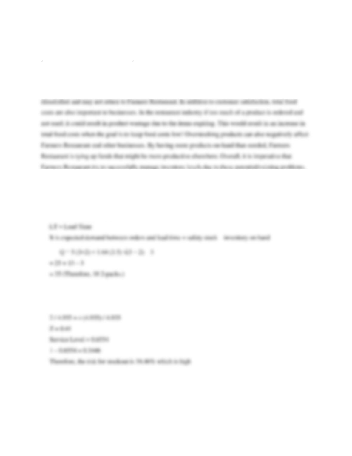
3. Q = ˉd (OI + LT) + zσd √(OI + LT) – A
OI = Time between orders
4. 12 = 5 x 2 + z (3.5) (1.41)
12 = 10 + z (4.935)
Chapter 13 – Inventory Management
13-34
Operations Tour: Bruegger’s Bagel Bakery
1. If too little inventory is maintained, there is a risk of stockout and potential lost sales. In addition,
2. a. Customers judge the quality of bagels by their appearance (size, shape and shine), taste and
consistency. Customers are also very interested in receiving high service quality.
b. At each stage of the production process, workers check bagel quantity.
c. Steps for Bruegger’s Bagel Bakery Operations:
a. Purchase ingredients from suppliers
b. Mix the dough
c. Shape the dough
The company can improve quality at each step by monitoring output more carefully and training
and education of the employees.
3. The basic ingredients can be purchased using either fixed order interval or fixed order quantity
4. If there is a bagel-making machine at each store, the company would have to invest in more
Enrichment Module: Advanced EOQ Problem
This enrichment module consists of an additional EOQ problem to further solidify the concepts associated
with the Economic Production Model. The question forces the students to work backwards through the
EOQ production equation.
Problem
A company produces plastic powder in lots of 2000 pounds, at the rate of 250 pounds per hour. The
Chapter 13 – Inventory Management
13-35
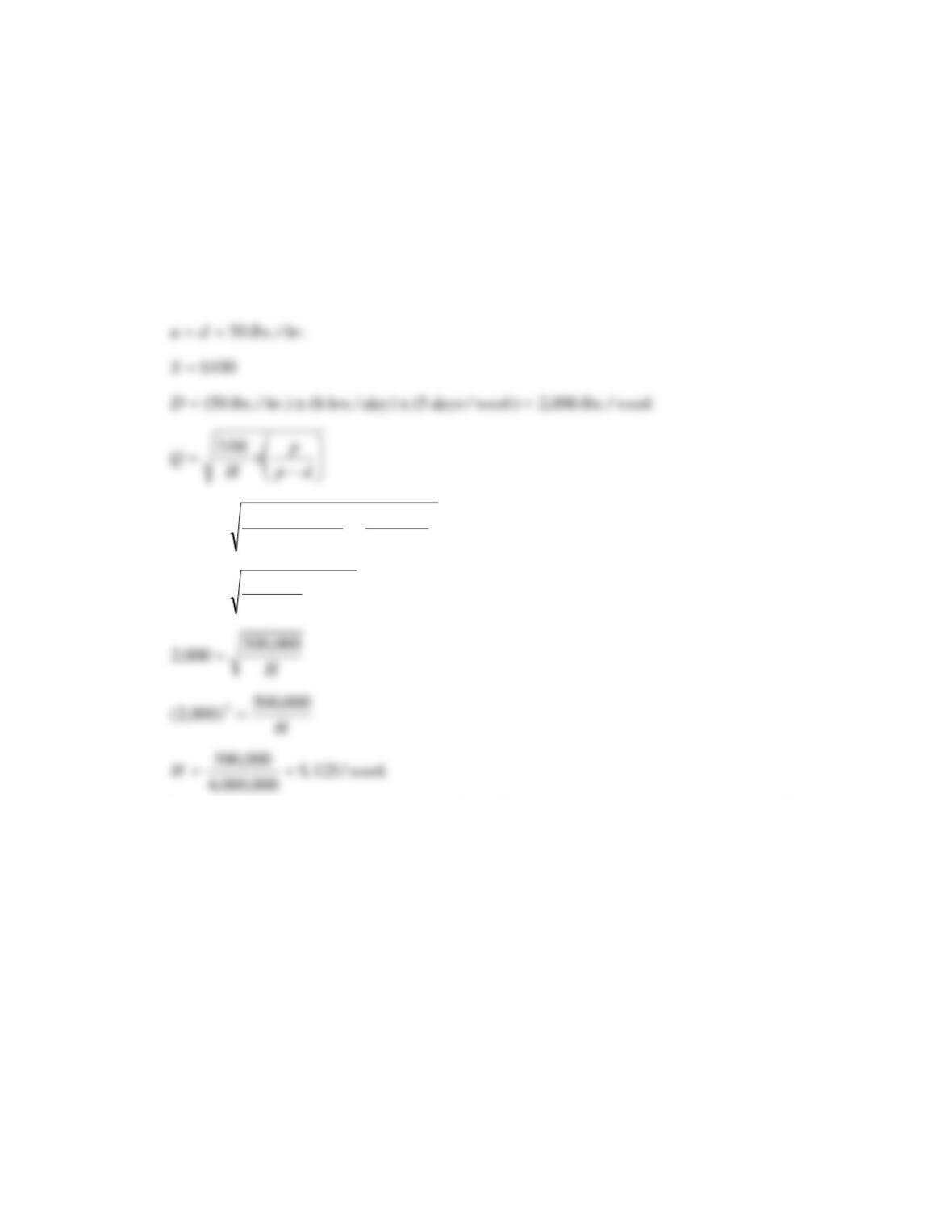
a. What weekly holding cost per pound does the lot size imply, assuming the lot size is optimal?
b. Suppose the figure you compute for holding cost has been shown to the manager, and the
manager says that it is not that high. Would that mean the lot size is too large or too small?
Explain.
Solution to Enrichment Module Problem
a.
H
H
hrlbs p
lbs Q
)25.1x(
000,400
000,2
50250
250
x
)100)(000,2(2
000,2
./.250
.000,2
=
−
=
=
=
b. Decreasing the value of carrying cost (H) will result in an increase in the lot size. Since
holding inventory is not as expensive, the firm can afford to carry more inventory and
therefore produce a larger batch.
Chapter 13 – Inventory Management
13-36
Enrichment Module 2: Inventory Model with Planned Shortages
In most cases, shortages are undesirable and should be avoided. However, in certain circumstances, it
may be desirable to plan and allow for shortages. Planned shortages are implemented for high dollar
form of backorders. In many cases the cost of backorders can be easily offset by the reduction in carrying
costs. The model discussed in this section will not be valid if a customer decides not to wait for the
backorder.
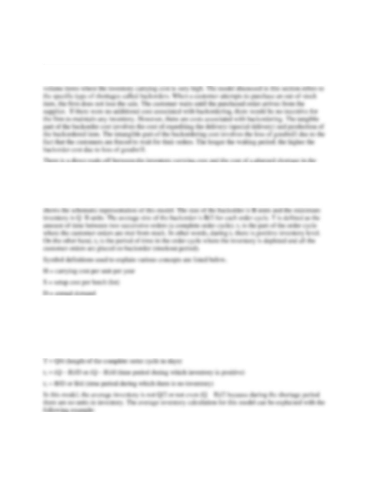
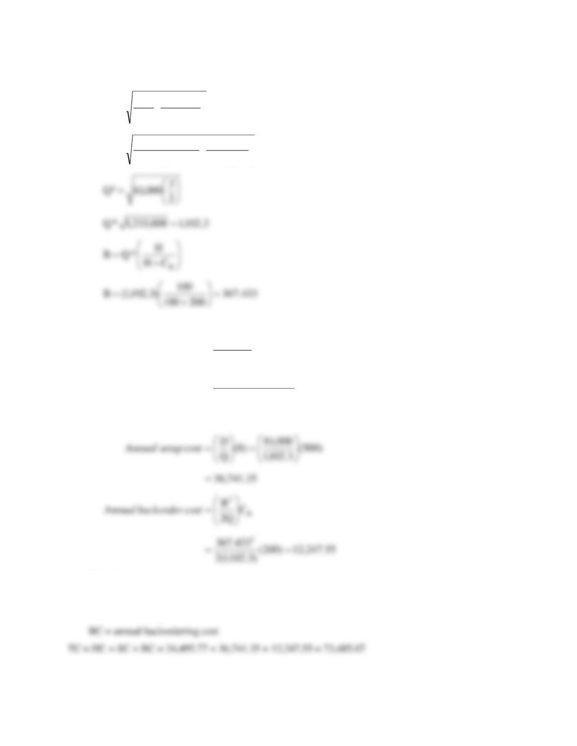
The fixed order quantity inventory model with planned shortages (backorders) is very similar to the basic
EOQ model. When the reorder point is reached, a new economic order quantity (Q) is placed. Figure 1
Q* = optimal order quantity
B = size of the backorder
CB = backorder cost per unit per year
B* = optimal planned backorder quantity
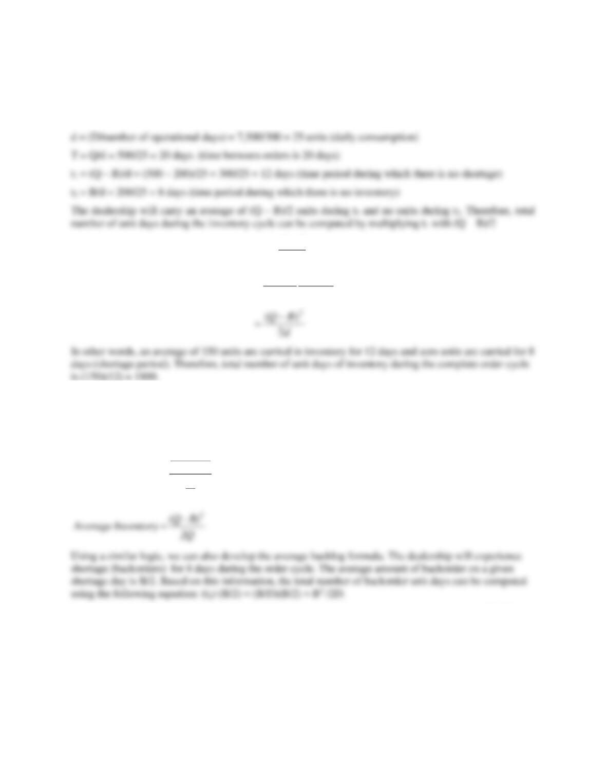
T = Q/D (length of the complete order cycle in years) or
Chapter 13 – Inventory Management
13-37
A large local car dealership orders a certain brand of automobiles from a car manufacturer located in
Detroit. Order quantity (Q) is 500 units, annual demand (D) is 7500 and the firm operates 300 working
days per year. Due to the high holding costs, the company plans to backorder (B) 200 cars per order cycle.
Determine the average inventory.
BQ
d
B)(Q
cycleinventory/ of days unit of Number
BQ
tcycleinventory/ of days unit of Number
2
)(
2
*
1
−−
=
−
=
Since there are a total of 20 days in the complete order cycle, the average inventory can be computed by
dividing the total number of unit days of inventory by the number of days in the inventory cycle. In this
example, the average inventory is equal to 1,800/20 or 90 units. Therefore, the average inventory can be
computed by using the following formula:
d
Q
d
BQ
inventory Average
−
=2
)( 2
In our example, there are 8 days of a planned shortage period. During this period, an average of 200/2 =
100 units of backorders are realized. Therefore, the total number of backorder unit days during the order
cycle is (8)(100) = 800 units. Since there are a total of 20 days in the order cycle, the average backorder
quantity for the complete order cycle can be determined by dividing the total number of backorder unit
days by the number of days in the complete inventory cycle. In this example, using the above equation,
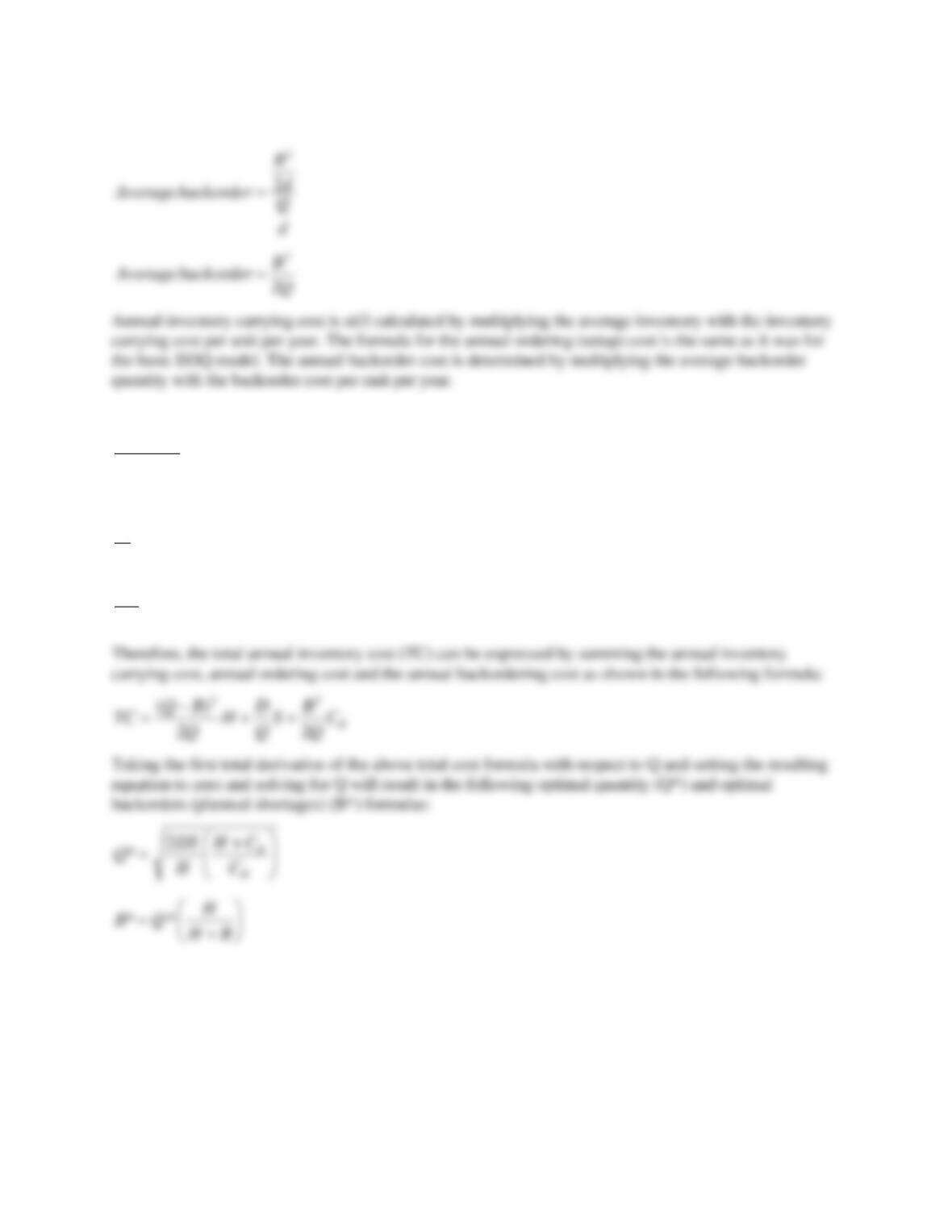
we obtain an average backorder quantity of 800/20 = 40 units. The general equation for the average
backorder quantity is:
Chapter 13 – Inventory Management
13-38
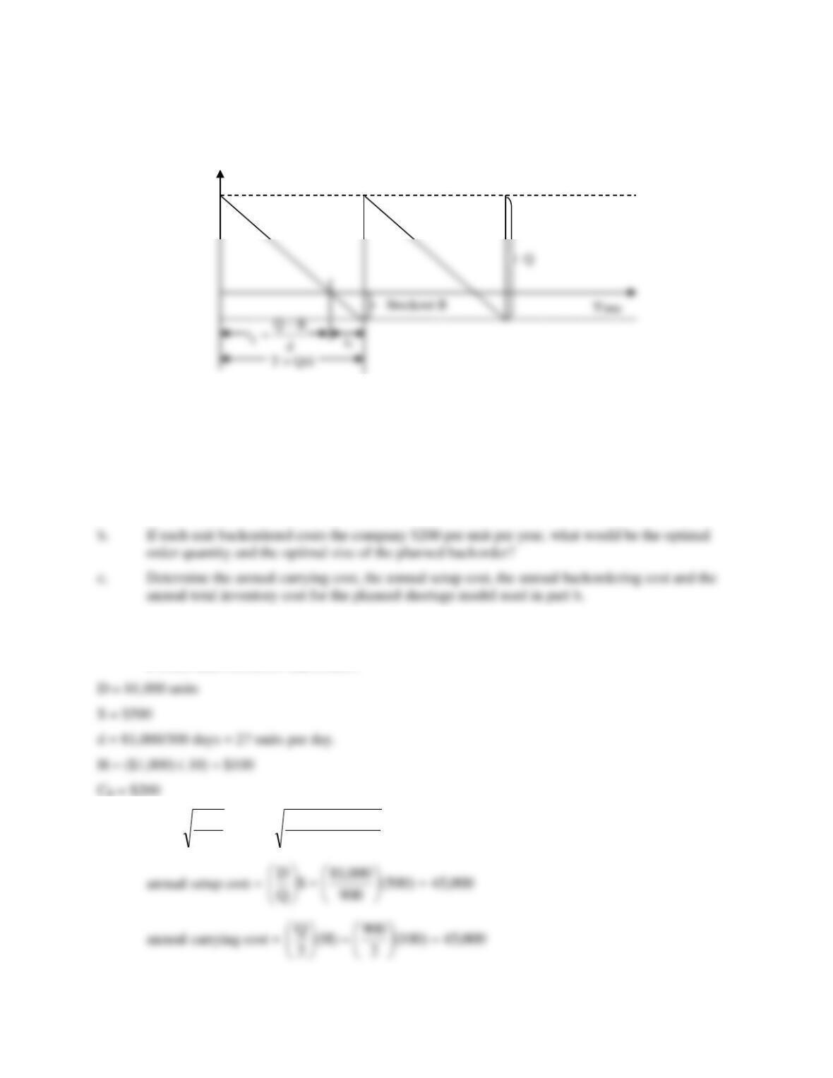
The annual inventory carrying cost is given by:
H
Q
BQ
2
)( 2
−
The annual ordering and backordering costs are given by the following respective formulas:
B
C
Q
B
S
Q
D
2
2
Chapter 13 – Inventory Management
13-39
Figure 1
An inventory situation with planned shortages
Example:
XYZ Company distributes a major part for the F–15 fighter jets. Due to the very high holding cost, the
company wants to implement a model with planned shortages. The annual demand is 78,000 and the
company operates 300 days per year. The annual carrying rate is 10% of the item cost and the unit cost of
this item is $1,000. The setup cost per batch is estimated at $500.
a. Determine the optimal order quantity and total annual inventory cost (setup cost + carrying cost)
using the basic EOQ model with no backorders.
d. Determine the values of t1, t2 and T in days.
e. Should the company adopt the planned backorder model of part b or the basic EOQ model of part
a which does not allow backorders?
a.
900
100
)500)(000,81(2
Q*
H
DS2
*Q ===
Inventory
Q – B
Maximum Inventory Level
Chapter 13 – Inventory Management
13-40
200
200100
H
)500)(000,81(2
*Q
C
)CH(
H
DS2
*Q
B
B
+
=
+
=
c.
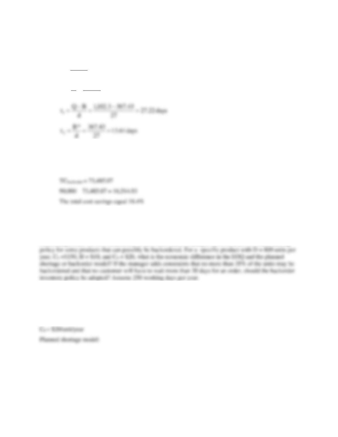
77.495,24
)100(
)3.102,1(2
)43.3673.102,1(
H
Q2
)BQ(
2
2
=
−
=
−
=
cost carrying Annual
Let TC = Total annual inventory cost
HC = annual inventory holding cost
SC = annual setup cost
Chapter 13 – Inventory Management
13-41
d.
days83.40
27
3.102,1
d
Q
T
27
300
000,81
d
===
==
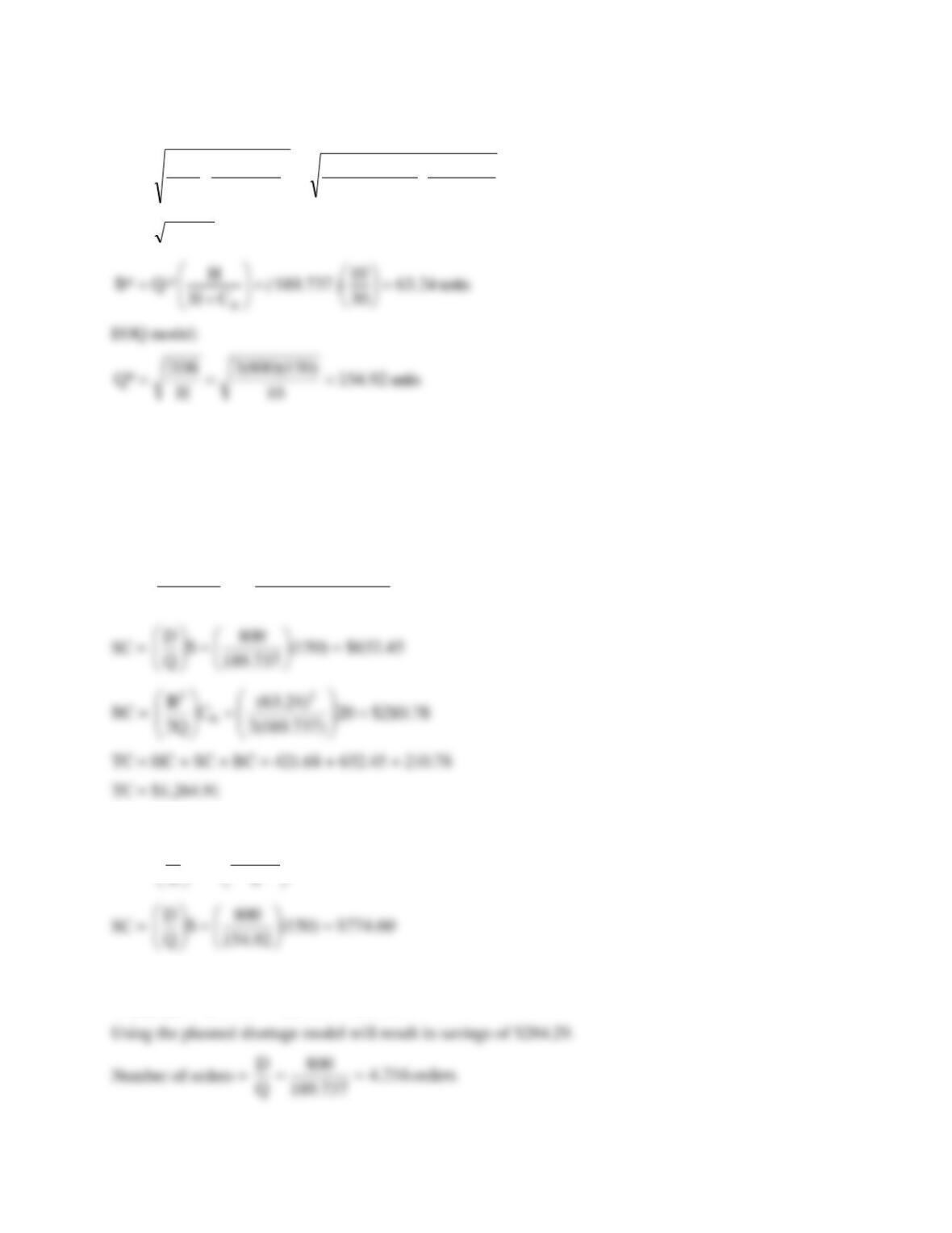
e. The model with planned backorders is preferred because the total annual inventory cost of the
basic inventory model is substantially higher than the total annual inventory cost of the planned
backorder model.
TCbasic EOQ = 90,000
Problems
The manager of an inventory system believes that inventory models are important decision-making aids.
Although the manager often uses an EOQ policy, he has never considered a backorder model because of
his assumption that backorders are “bad” and should be avoided. However, with upper management’s
continued pressure for cost reduction, you have been asked to analyze the economics of a backordering
Solution to Problem
D = 800 units/year
C0 = $150
H = $10/unit/year
Chapter 13 – Inventory Management
13-42
units 73718900092Q
20
2010
10
1508002
C
CH
H
DS2
Q
B
B
.,*
)())(()(
*
==
+
=
+
=
Total cost planned shortage model:
TC = Total annual inventory cost
HC = Annual inventory holding cost
SC = Annual setup cost
BC = Annual backordering cost
HC =
68.421$)10(
)737.189(2
)24.63737.189(
H
Q2
)BQ( 22
=
−
=
−
Total cost regular EOQ model:
HC =
60.774$)10(
92.154
H
Q=
=
TC = HC + SC = 774.60 + 774.60 =$1,549.20
TCDifference = 1,549.20 – 1,264.91 = $284.29
Chapter 13 – Inventory Management
13-43
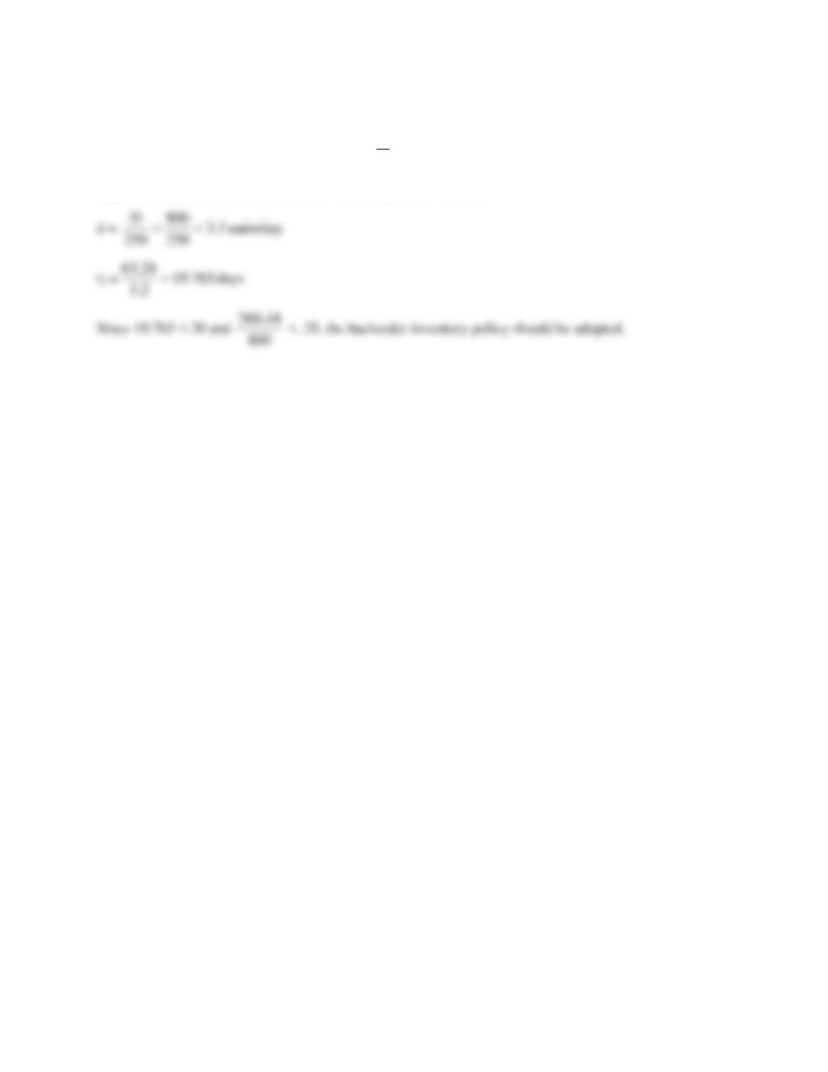
Expected annual number of units short = (B)
Q
D
Expected annual number of units short = (63.24)(4.216) = 266.44