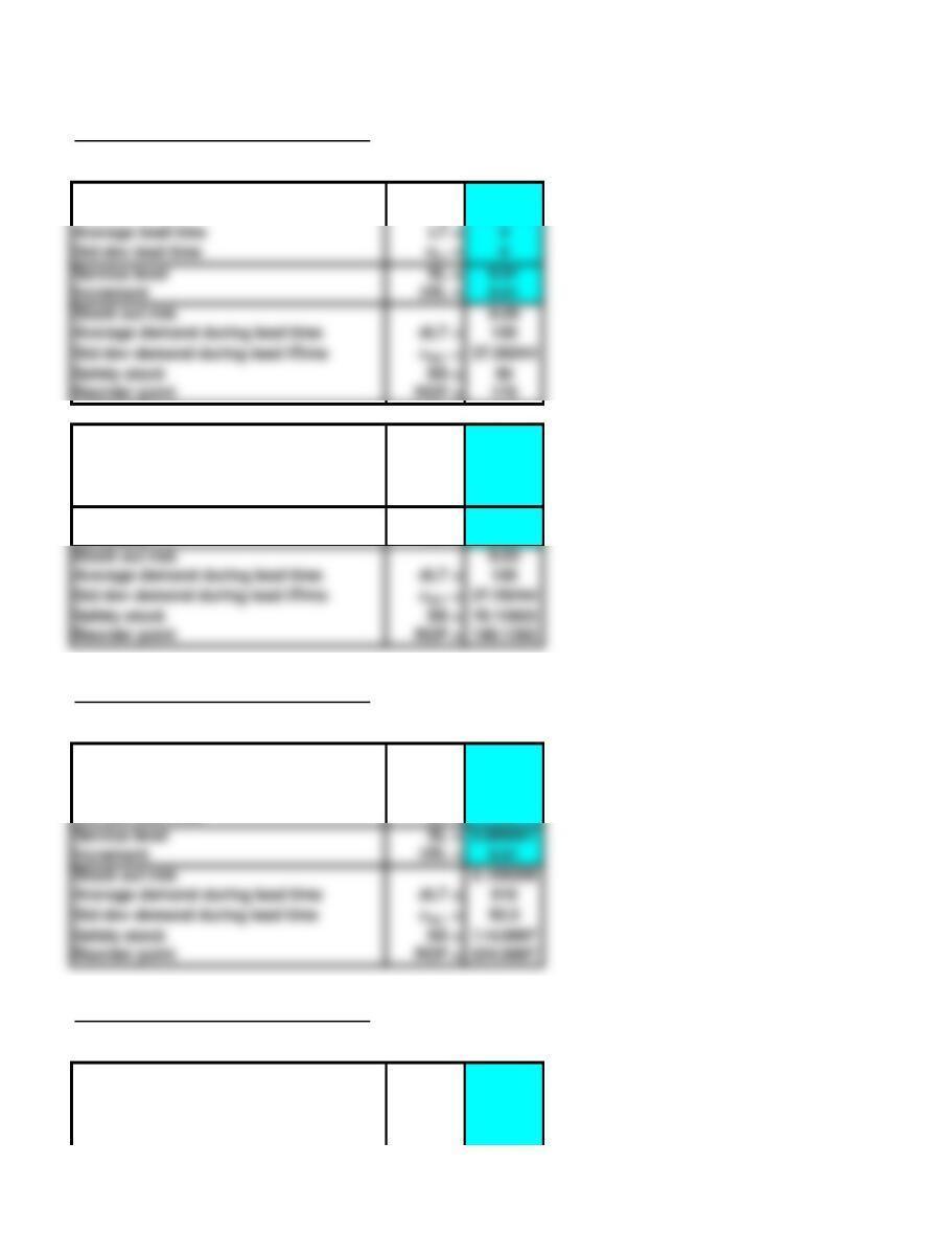
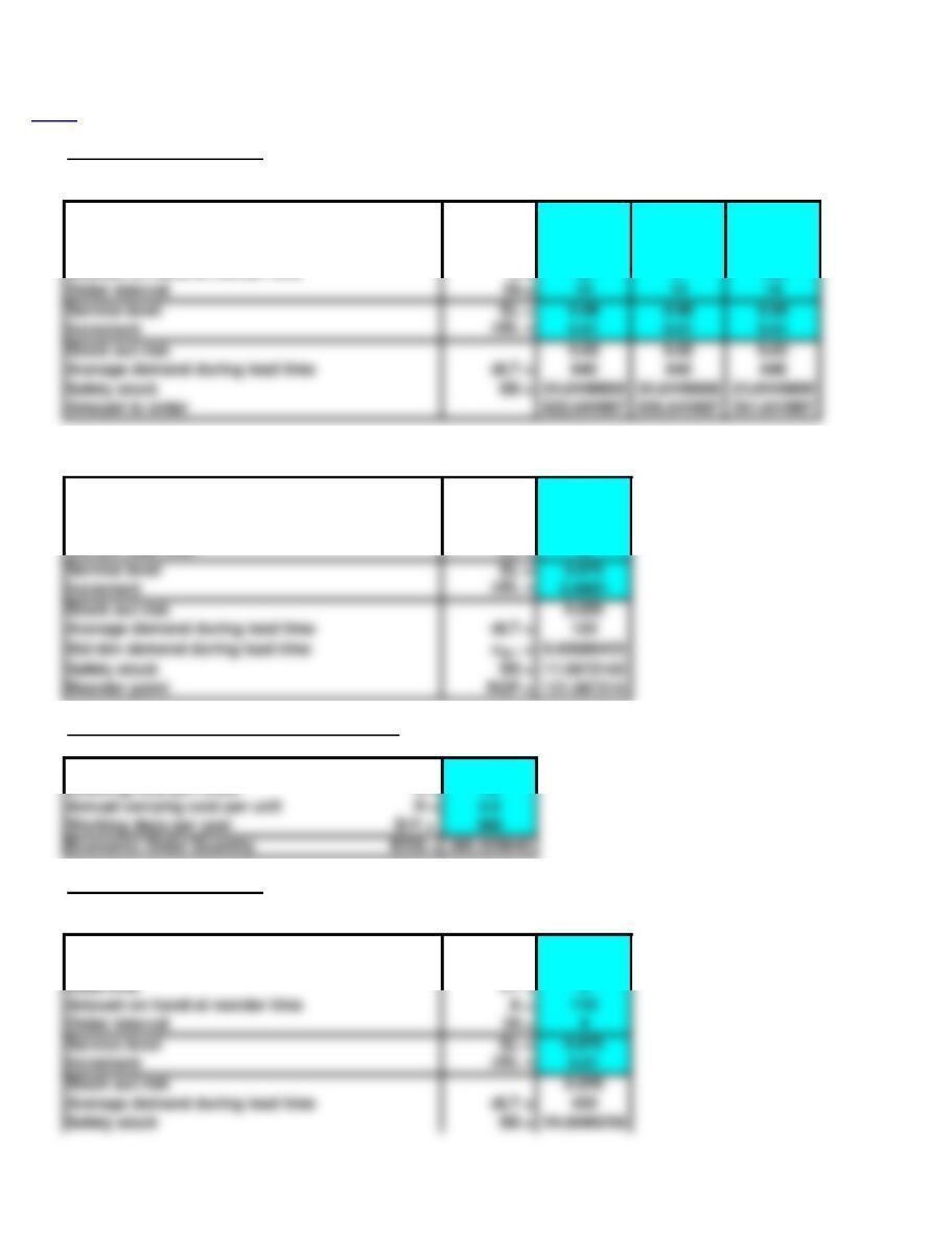
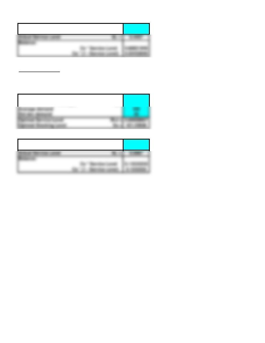
22. Reorder Point (ROP) with EOQ Ordering
Average demand d = 30
Std dev demand
sd = 18.64622
Average demand d = 30
Std dev demand
sd = 18.64622
Average lead time LT = 4
Std dev lead time
sLT = 0
Service level SL = 0.97
Increment DSL = 0.01
Stock out risk 0.03
Average demand during lead time dLT = 120
Safety stock SS = 70.13923
23. Reorder Point (ROP) with EOQ Ordering
Average demand d = 85
Std dev demand
sd = 0
Average lead time LT = 6
Std dev lead time
sLT = 1.1
Service level SL = 0.890641
Increment DSL = 0.01
Stock out risk 0.109359
Average demand during lead time dLT = 510
Safety stock SS = 114.9997
24. Reorder Point (ROP) with EOQ Ordering
Average demand d = 12
Std dev demand
sd = 2
Average lead time LT = 4
Std dev lead time
sLT = 1
Average lead time LT = 4
sLT = 0
Service level SL = 0.91
Increment DSL = 0.01
Stock out risk 0.09
Average demand during lead time dLT = 120
Service level SL = 0.96
Increment DSL = 0.01
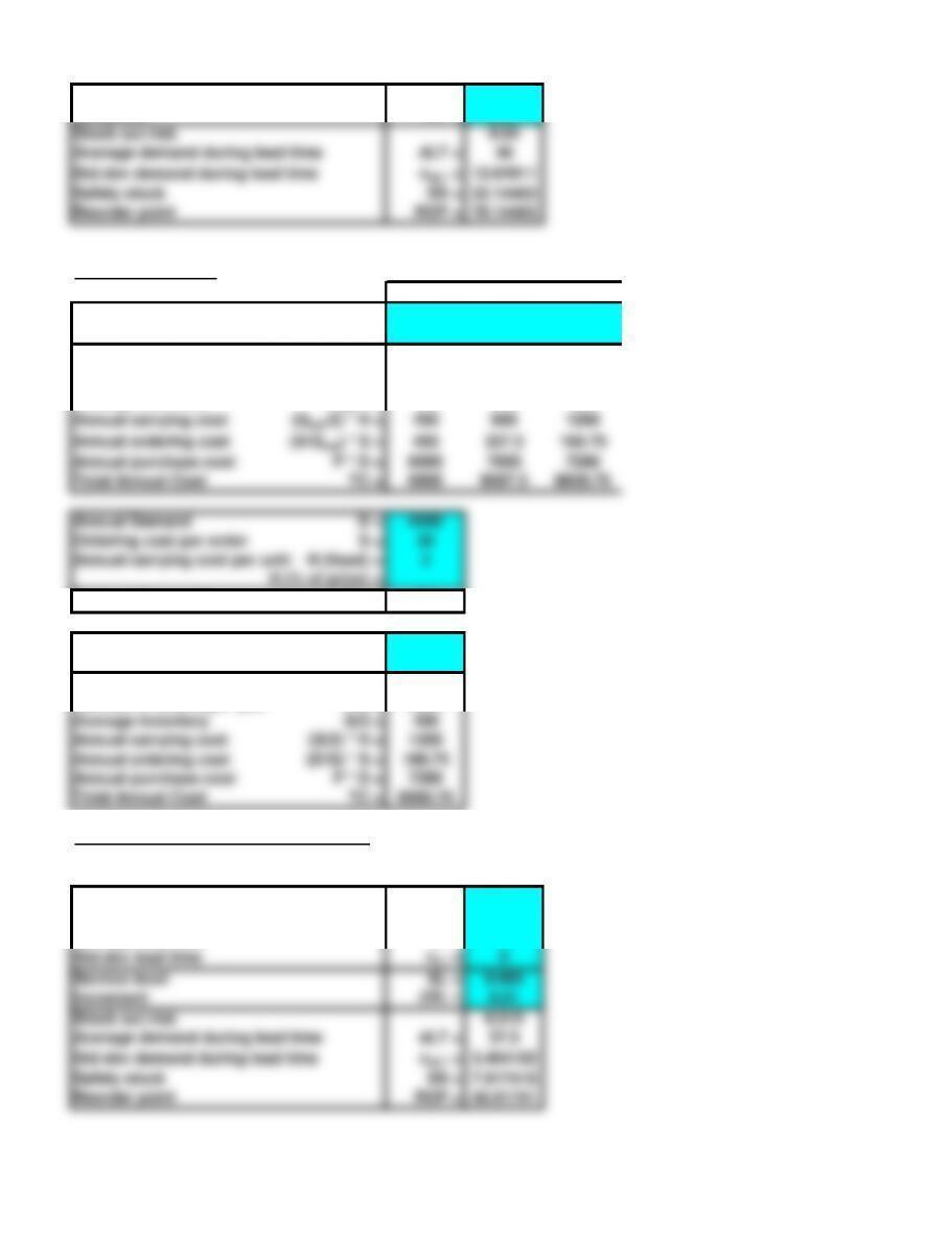
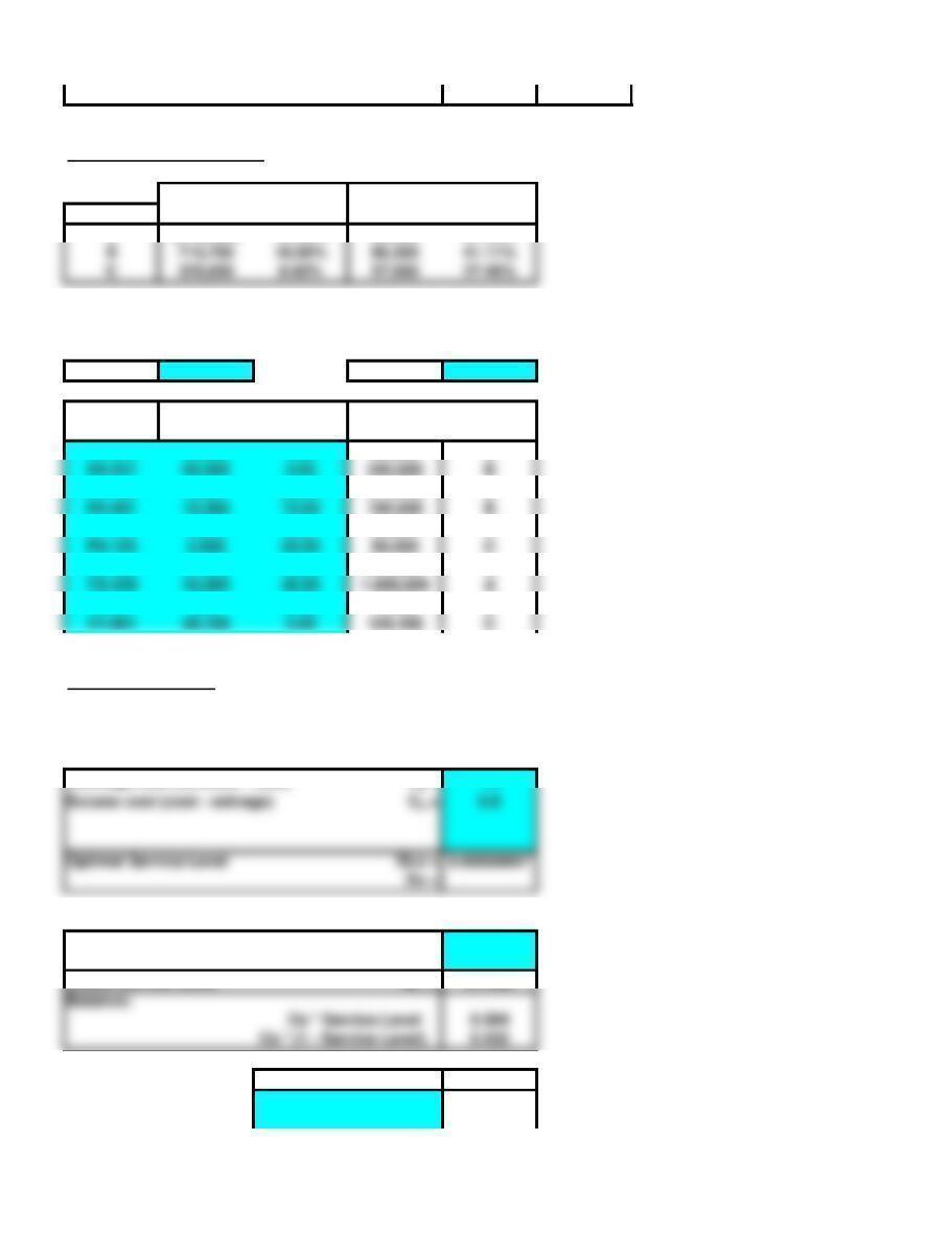
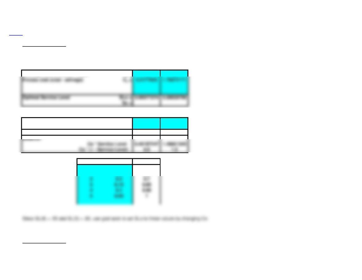
25a. Quantity Discounts
Price Level: 1 2 3
Minimum quantity for price
Qmin = 1400 800
Price P = 2.00 1.70 1.62
Optimal Q (for each price)
Qopt = 300 400 800
Number of orders per year
D/Qopt = 15 11.25 5.625
Average Inventory
Qopt/2 = 150 200 400
Annual purchase cost P * D = 9000 7650 7290
Total Annual Cost TC = 9900 8587.5 8658.75
Annual Demand D = 4500
Ordering cost per order S = 30
Annual carrying cost per unit: H (fixed) = 3
Optimal Q (overall)
Qopt = 400
Actual Order Quantity Q = 800
Increment DQ = 10
Price P = 1.62
Number of orders per year D/Q = 5.625
Annual ordering cost (D/Q) * S = 168.75
Annual purchase cost P * D = 7290
Total Annual Cost TC = 8658.75
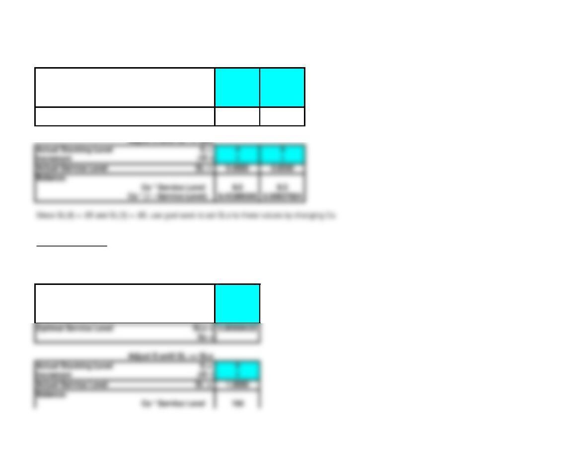
25b. Reorder Point (ROP) with EOQ Ordering
Average demand d = 12.5
Std dev demand
sd = 2
Average lead time LT = 3
Service level SL = 0.985
Stock out risk 0.015
Average demand during lead time dLT = 37.5
Safety stock SS = 7.517415
Stock out risk 0.04
Average demand during lead time dLT = 48
Safety stock SS = 22.14463
Reorder point ROP = 70.14463
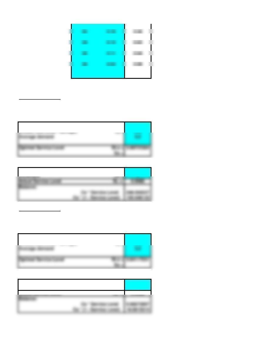
26a. Basic Economic Order Quantity (EOQ) Model
Annual Demand D = 260
Ordering cost per order S = 2
26b. Reorder Point (ROP) with EOQ Ordering
Average demand d = 5
Std dev demand
sd = 0.5
Average lead time LT = 2
Std dev lead time
sLT = 0
Service level SL = 0.997669
Stock out risk 0.002331
Average demand during lead time dLT = 10
Safety stock SS = 2.000792
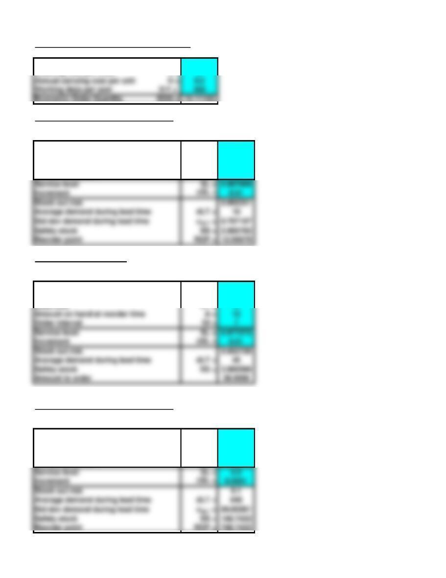
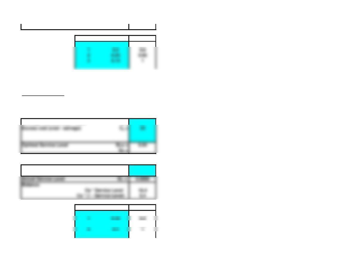
26c. Fixed Order Interval Model
Average demand d = 5
Std dev demand
sd = 0.5
Lead time LT = 2
Amount on hand at reorder time A = 12
Service level SL = 0.977272
Stock out risk 0.022728
Average demand during lead time dLT = 45
Safety stock SS = 3.000596
27. Reorder Point (ROP) with EOQ Ordering
Average demand d = 80
Std dev demand
sd = 10
Average lead time LT = 8
Std dev lead time
sLT = 1
Service level SL = 0.9
Stock out risk 0.1
Average demand during lead time dLT = 640
Safety stock SS = 108.7432
Annual carrying cost per unit H = 0.2
28a. Basic Economic Order Quantity (EOQ) Model
Annual Demand D = 3600
Ordering cost per order S = 1
28b. Reorder Point (ROP) with EOQ Ordering
Average demand d = 10
Std dev demand
sd = 2
Average lead time LT = 3
Service level SL = 0.96
Stock out risk 0.04
Average demand during lead time dLT = 30
Safety stock SS = 6.064555
Annual carrying cost per unit H = 0.4
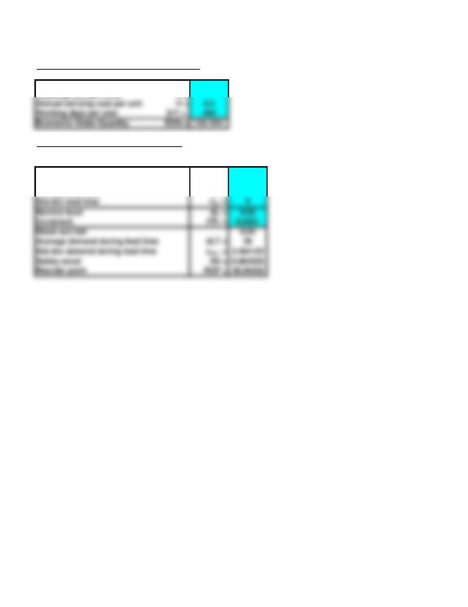
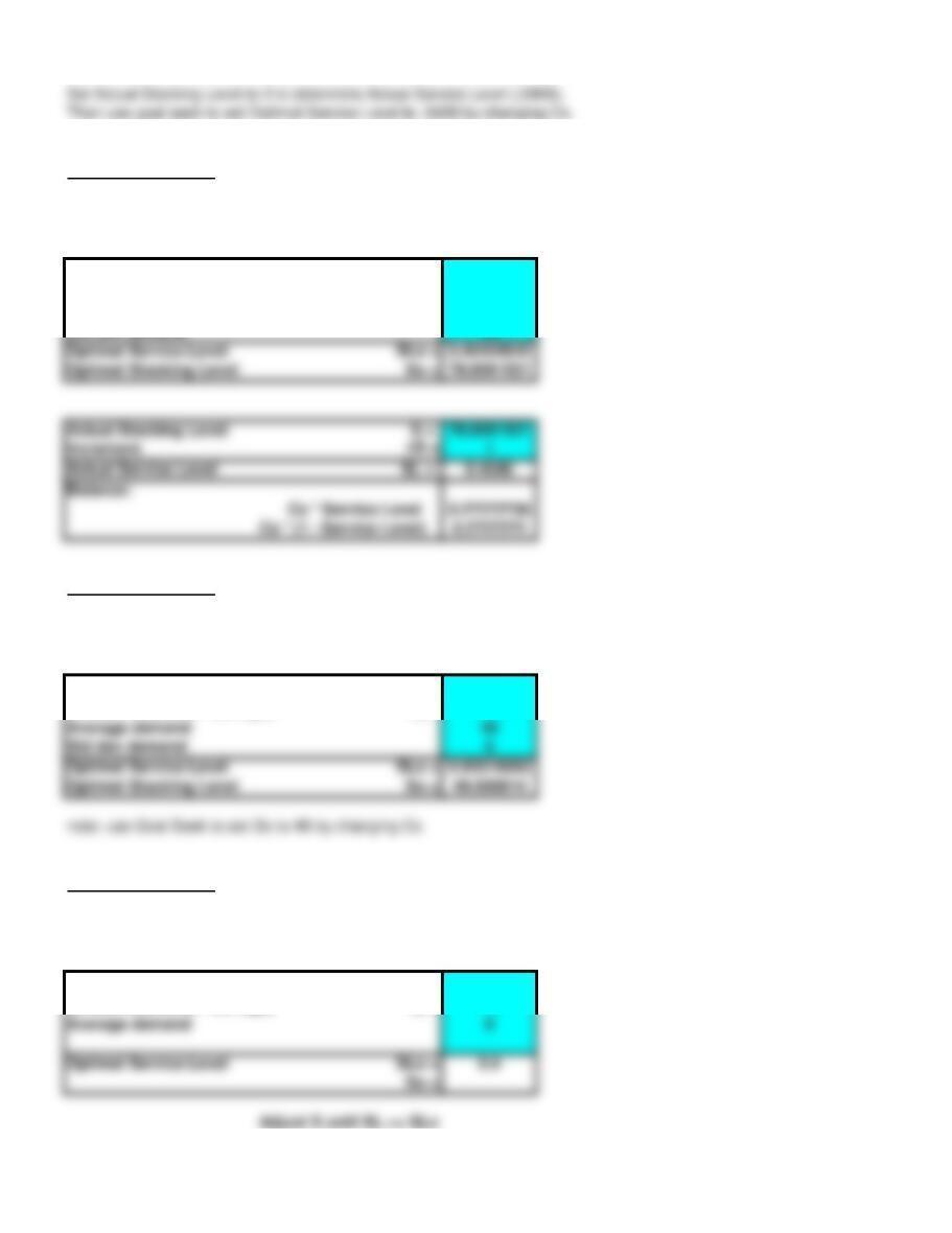
Chapter 13 – Problems 31-39 Note: This worksheet displays results only, you must copy the shaded
<Back area into the corresponding template to make additional calculations.
31. Fixed Order Interval Model
Average demand d = 40 40 40
Std dev demand
sd = 3 3 3
Lead time LT = 2 2 2
Amount on hand at reorder time A = 42 8103
32a. Average demand d = 60
Std dev demand
sd = 4
Average lead time LT = 2
Std dev lead time
sLT = 0
Service level SL = 0.975
Stock out risk 0.025
Average demand during lead time dLT = 120
Safety stock SS = 11.0872142
32b. Basic Economic Order Quantity (EOQ) Model
Annual Demand D = 3000
Ordering cost per order S = 70
Annual carrying cost per unit H = 4.5
32c. Fixed Order Interval Model
Average demand d = 70
Std dev demand
sd = 5
Lead time LT = 2
Amount on hand at reorder time A = 110
Service level SL = 0.975
Stock out risk 0.025
Average demand during lead time dLT = 420
Safety stock SS = 24.0045228
Service level SL = 0.98 0.98 0.98
Stock out risk 0.02 0.02 0.02
Average demand during lead time dLT = 640 640 640
Safety stock SS = 24.6449869 24.6449869 24.6449869
Amount to order 334.004523
33a. ABC Classification Syatem
Dollar Amount Annual Demand
Class Total Percent Total Percent
A2,745,000 72.50% 66,000 31.44%
Enter lower limit for dollar amount:
A945,000 B195,600
Unit Dollar
Item Usage Cost Amount Class
H4-010 20,000 2.50 50,000 C
H5-201 60,200 4.00 240,800 B
P6-400 9,800 28.50 279,300 B
P7-100 6,250 9.00 56,250 C
P9-103 4,500 22.00 99,000 C
TS-300 21,000 45.00 945,000 A
TS-400 45,000 40.00 1,800,000 A
TS-041 800 20.00 16,000 C
34. Single Period Model
Select demand distribution: Discrete
4
Shortage cost (revenue – cost)
Cs = 1.6
Ce = 0.8
Adjust S until SL >= SLo
Actual Stocking Level S = 25
Increment DS = 1
Actual Service Level SL = 0.7300
Cs * (1 – Service Level) 0.432
Discrete Distribution: Demand Freq Cum
19 0.01 0.01
20 0.05 0.06
21 0.12 0.18
23 0.13 0.49
24 0.14 0.63
25 0.1 0.73
26 0.11 0.84
27 0.1 0.94
28 0.04 0.98
29 0.02 1
35a. Single Period Model
Select demand distribution: Poisson
FALSE FALSE TRUE
Shortage cost (revenue – cost)
Cs = 88000
Excess cost (cost – salvage)
Ce = 245
Average demand 3.2
Adjust S until SL >= SLo
Actual Stocking Level S = 9
Increment DS = 1
Cs * (1 – Service Level) 155.046132
35b. Single Period Model
Select demand distribution: Poisson
FALSE FALSE TRUE
Shortage cost (revenue – cost)
Cs = 10.5203647
Excess cost (cost – salvage)
Ce = 245
Average demand 3.2
Adjust S until SL >= SLo
Actual Stocking Level S = 0
Increment DS = 1
36. Single Period Model
Select demand distribution: Normal
FALSE TRUE FALSE
Shortage cost (revenue – cost)
Cs = 0.5
Excess cost (cost – salvage)
Ce = 0.6
Average demand 80
Std dev demand 10
Optimal Stocking Level So = 78.8581521
Actual Stocking Level S = 78.8581521
Actual Service Level SL = 0.4545
37. Single Period Model
Select demand distribution: Normal
FALSE TRUE FALSE
Shortage cost (revenue – cost)
Cs = 4.88895816
Excess cost (cost – salvage)
Ce = 0.35
Average demand 40
Std dev demand 6
Optimal Stocking Level So = 49.000014
38. Single Period Model
Select demand distribution: Poisson
Shortage cost (revenue – cost)
Cs = 1
Excess cost (cost – salvage)
Ce = 1.5
Average demand 6
Actual Stocking Level S = 5
Increment DS = 1
39. Single Period Model
Select demand distribution: Normal
Shortage cost (revenue – cost)
Cs = 0.4
Excess cost (cost – salvage)
Ce = 0.2
Average demand 400
Actual Stocking Level S = 421.53638
Increment DS = 1
Chapter 13 – Problems 40-44 Note: This worksheet displays results only, you must copy the shaded
<Back area into the corresponding template to make additional calculations.
40a. Single Period Model
Select demand distribution: Discrete
4
Shortage cost (revenue – cost)
Cs = 10 10
Adjust S until SL >= SLo
Actual Stocking Level S = 4 3
Increment DS = 1 1
Actual Service Level SL = 0.9500 0.8500
Cs * (1 – Service Level) 0.5 1.5
Discrete Distribution: Demand Freq Cum
00.3 0.3
10.2 0.5
20.2 0.7
40.1 0.95
40b. Single Period Model
Ce = 0.5177605 1.76072171
Select demand distribution: Discrete
Shortage cost (revenue – cost)
Cs = 189.077861 56.7225216
Excess cost (cost – salvage)
Ce = 10 10
Optimal Service Level SLo = 0.9497684 0.85012557
So =
41. Single Period Model
Select demand distribution: Discrete
4
Shortage cost (revenue – cost)
Cs = 1000
Excess cost (cost – salvage)
Ce = 150
So =
Actual Stocking Level S = 3
Actual Stocking Level S = 4 3
Cs * (1 – Service Level) 0
Discrete Distribution: Demand Freq Cum
00.1 0.1
Since SL(2) = .85 and SL(3) = 1.0, stock 3 spares.
42b. Single Period Model
Select demand distribution: Discrete
4
Shortage cost (revenue – cost)
Cs = 27
Ce = 23
Adjust S until SL >= SLo
Actual Stocking Level S = 2
Increment DS = 1
Actual Service Level SL = 0.8000
Cs * (1 – Service Level) 5.4
Discrete Distribution: Demand Freq Cum
00.15 0.15
10.35 0.5
20.3 0.8
30.2 1
10.5 0.6
20.25 0.85
30.15 1
Since SL(1) = .5 and SL(2) = .8, stock 2 cakes.
43. Single Period Model
Select demand distribution: Normal
Shortage cost (revenue – cost) Cs = 99
Excess cost (cost – salvage) Ce = 200
Average demand 18
Actual Stocking Level S = 16.0122523
44. Reorder Point (ROP) with EOQ Ordering
Average demand d = 4.6
Std dev demand sd = 1.265
Average lead time LT = 3
Service level SL = 0.97238026
Stock out risk 0.02761974
Average demand during lead time dLT = 13.8
Std dev demand during lead time sdLT = 2.19104427
Safety stock SS = 4.2002052
Optimal Service Level SLo = 0.33110368
Use Goal Seek to set ROP = 18