Excel Templates to accompany Operations Management, Eleventh Edition
created by Lee Tangedahl
Copyright © 2012 by The McGraw Hill Companies, Inc. All rights reserved.
Chapter Thirteen – Inventory Management
Example 13
Templates: ABC Classification System (B) Example 14a
Basic Economic Order Quantity (EOQ) Model (B) Example 14b
Solved Problems: Solved Problem 1
(B) – includes Basic template Solved Problem 2
Solved Problem 3
Lecture Suggestions Solved Problem 4
Solved Problem 5
Examples: Example 1 Solved Problem 6
Example 2 Solved Problem 8
Example 3 Solved Problem 9
Example 4
Example 5 Problems: Problems 1-10
Example 6 Problems 11-20
Example 7 Problems 21-28
Example 8 Problems 31-39
Example 9 Problems 40-44
See the Inventory Management tutorial for a demonstration of the these templates.
See Instructions template for complete instructions.
Economic Production Quantity (EPQ) Model (B) Example 15
Quantity Discounts (B) Example 16
Reorder Point (ROP) with EOQ Ordering (B) Example 17
Fixed Order Interval Model (B) Example 18
Single Period Model (B)
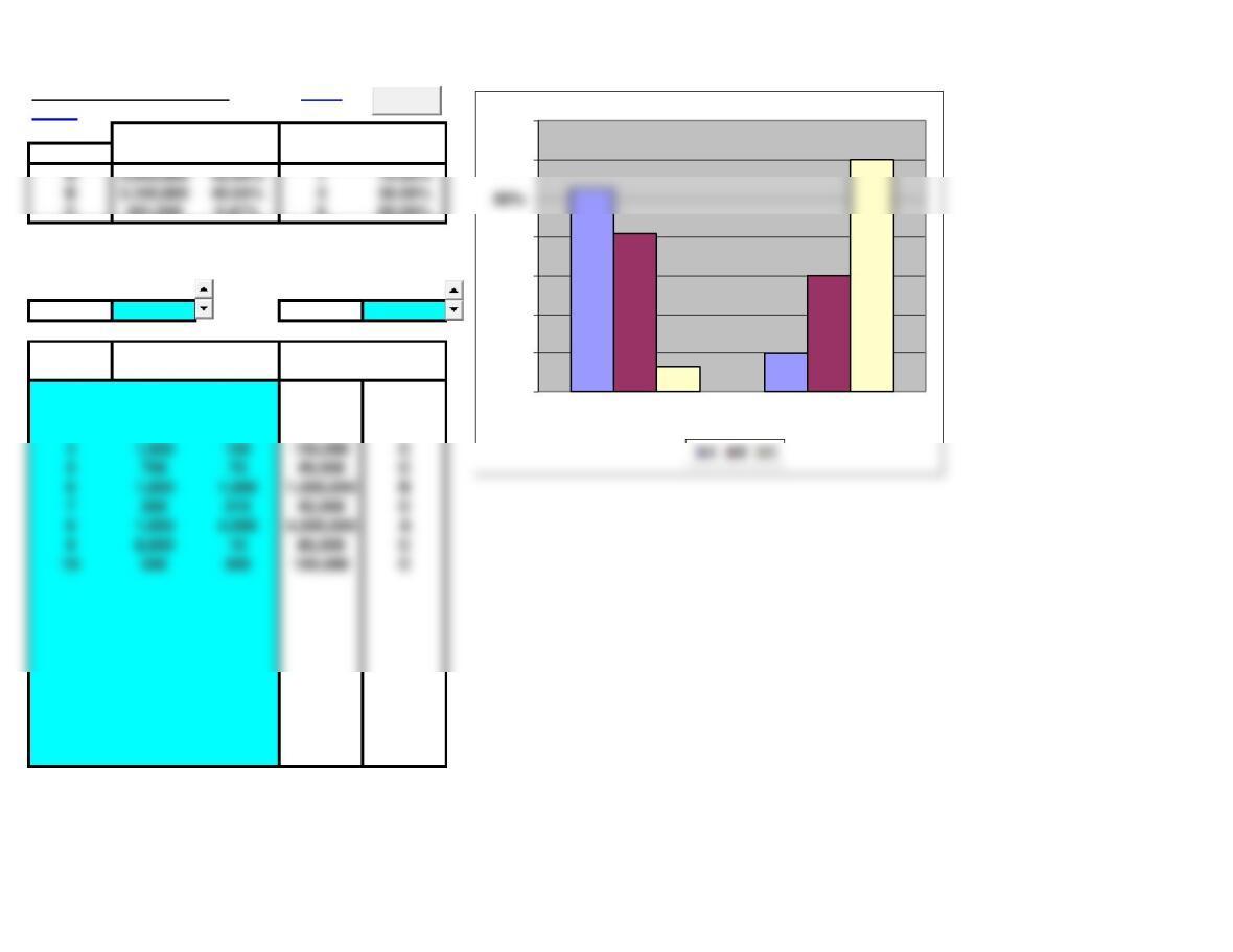
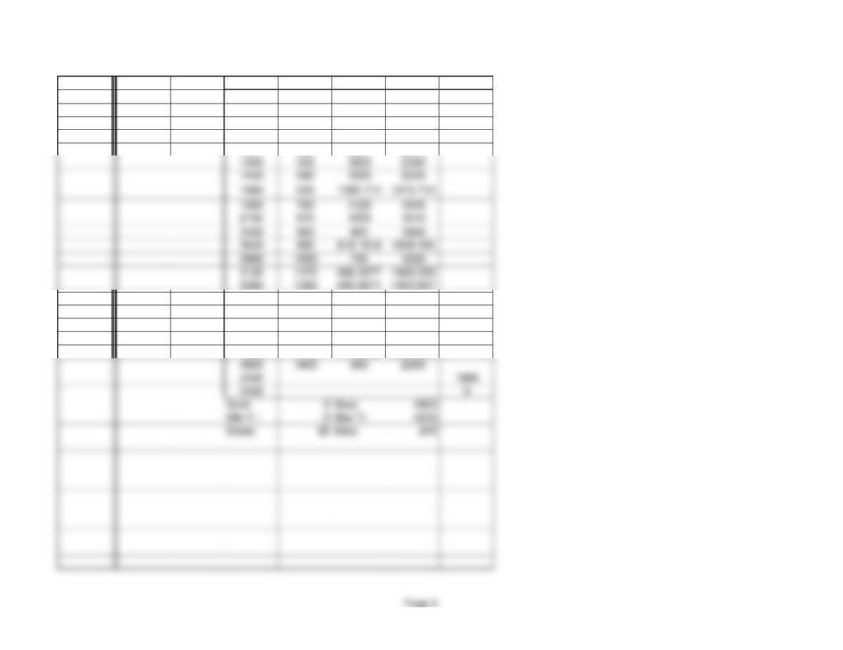
ABC Classification System Basic
<Back
Dollar Amount Number of Items
Class Total Percent Total Percent
C491,000 6.47% 660.00%
Enter lower limit for dollar amount:
A4,000,000 B900,000
Unit Dollar
Item Usage Cost Amount Class
12,500 360 900,000 B
21,000 70 70,000 C
32,400 500 1,200,000 B
41,500 100 150,000 C
61,000 1,000 1,000,000 B
81,000 4,000 4,000,000 A
98,000 10 80,000 C
0%
10%
20%
30%
40%
60%
70%
Dollar Amount Number of Items
Clear
Basic Template: You can simply copy the basic template below and paste into another worksheet.
^Top If you also copy the graph you will have to fix the cell references in the graph
(right-click on the graph, click Select Data…, and Edit the Series values for each series).
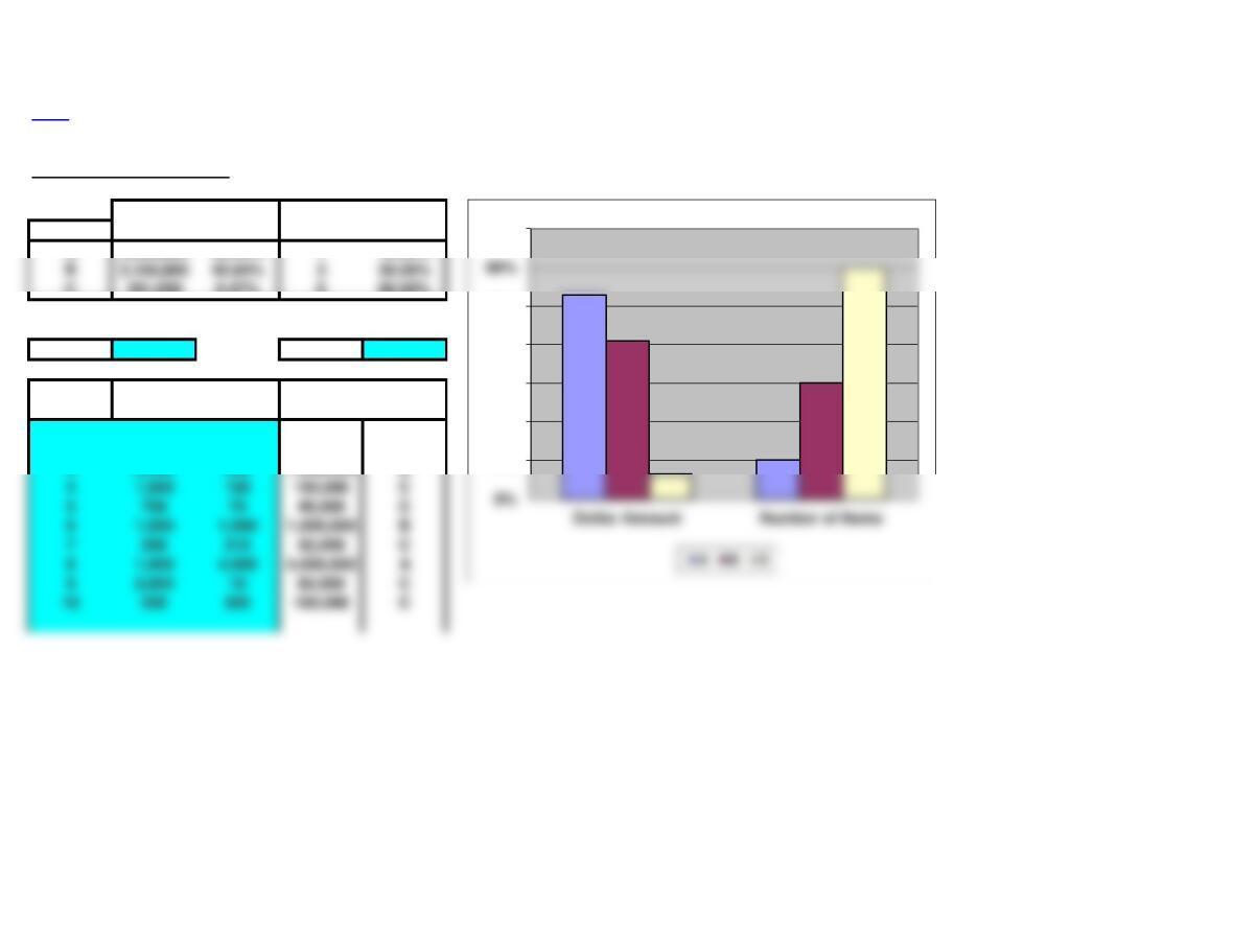
ABC Classification System
Dollar Amount Number of Items
Class Total Percent Total Percent
A4,000,000 52.69% 110.00%
C491,000 6.47% 660.00%
Enter lower limit for dollar amount:
A4,000,000 B900,000
Unit Dollar
Item Usage Cost Amount Class
12,500 360 900,000 B
21,000 70 70,000 C
32,400 500 1,200,000 B
41,500 100 150,000 C
61,000 1,000 1,000,000 B
81,000 4,000 4,000,000 A
98,000 10 80,000 C
10%
20%
30%
40%
50%
70%
EOQ
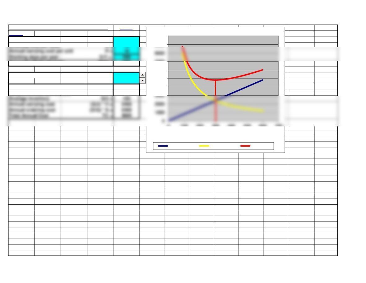
Basic Economic Order Quantity (EOQ) Model Basic
<Back
Annual Demand D = 9600
Ordering cost per order S = 75
Economic Order Quantity EOQ = 300
Actual Order Quantity Q = 300
Increment DQ = 10
Number of orders per year D/Q = 32
Length of order cycle (days) Q/D = 9
Average Inventory Q/2 = 150
Annual carrying cost (Q/2) * H = 2400
Annual ordering cost (D/Q) * S = 2400
Total Annual Cost TC = 4800
4,800.00
4000
5000
6000
7000
9000
10000
0100 200 300 400 500 600 700
Order Quantity (Q)
Carrying Cost Ordering Cost Total Cost
Page 4
Annual carrying cost per unit H = 16
Working days per year D/Y = 288
EOQ
Basic Template: You can simply copy the basic template below and paste into another worksheet.
^Top
Basic Economic Order Quantity (EOQ) Model
Annual Demand D = 9600
Ordering cost per order S = 75
Actual Order Quantity Q = 300
Number of orders per year D/Q = 32
Length of order cycle (days) Q/D = 11.25
Average Inventory Q/2 = 150
Annual carrying cost (Q/2) * H = 2400
Annual ordering cost (D/Q) * S = 2400
Page 5
EOQ
180 1440 4000 5440
210 1680 3428.571 5108.571
240 1920 3000 4920
270 2160 2666.667 4826.667
300 2400 2400 4800
300 4800
300 0
Start: 0 Stop: 600
Min Y : 0 Max Y: 9600
Steps: 20 Step: 30
150 1200 4800 6000
EPQ
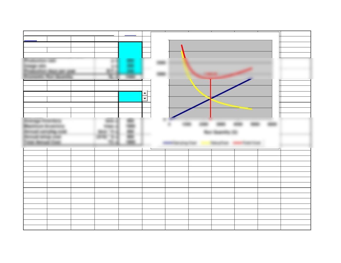
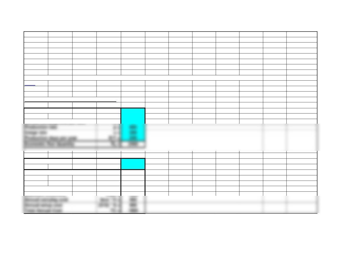
Economic Production Quantity (EPQ) Model Basic
<Back
Annual Demand D = 48000
Setup cost S = 45
Annual carrying cost per unit H = 1
Actual Run Quantity Q = 2400
Increment DQ = 100
Number of runs per year D/Q = 20
Cycle time Q/u = 12
Run time Q/p = 3
Average Inventory Iave = 900
Maximum Inventory Imax = 1800
Annual carrying cost Iave * H = 900
Annual setup cost (D/Q) * S = 900
500
1000
1500
3000
3500
Page 7
Production rate p = 800
Usage rate u = 200
EPQ
Basic Template: You can simply copy the basic template below and paste into another worksheet.
^Top
Economic Production Quantity (EPQ) Model
Annual Demand D = 48000
Setup cost S = 45
Annual carrying cost per unit H = 1
Actual Run Quantity Q = 2400
Increment DQ = 100
Number of runs per year D/Q = 20
Cycle time Q/u = 12
Run time Q/p = 3
Average Inventory Iave = 900
Maximum Inventory Imax = 1800
Annual carrying cost Iave * H = 900
Annual setup cost (D/Q) * S = 900
Page 8
Production rate p = 800
Usage rate u = 200
EPQ
x Carrying Setup Total Q
10.375 #N/A #N/A
240 90 #N/A #N/A
480 180 #N/A #N/A
720 270 3000 3270
960 360 2250 2610
3600 1350 600 1950
3840 1440 562.5 2002.5
4080 1530 529.4118 2059.412
4320 1620 500 2120
4560 1710 473.6842 2183.684
2640 990 818.1818 1808.182
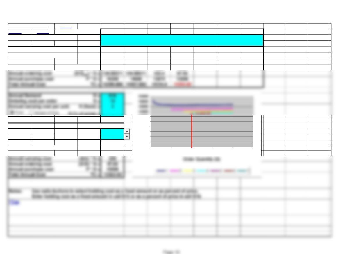
Quantity Discounts
Quantity Discounts Basic
<Back Notes Price Level: 1 2 3 4 5 6 7
Minimum quantity for price
Qmin = 150 80 100
Price P = 20.00 18.00 17.00 16.00
Optimal Q (for each price)
Qopt = 70 70 80 100
Number of orders per year
D/Qopt = 11.657143 11.657143 10.2 8.16
Average Inventory
Qopt/2 = 35 35 40 50
Annual carrying cost
(Qopt/2) * H = 140 140 160 200
1 TRUE H (% of price) =
Optimal Q (overall)
Qopt = 100
Actual Order Quantity Q = 100
Increment DQ = 10
Price P = 16
Number of orders per year D/Q = 8.16
Average Inventory Q/2 = 50
Annual ordering cost (D/Q) * S = 97.92
Annual purchase cost
Total Annual Cost TC = 13353.92
Notes: Use radio buttons to select holding cost as a fixed amount or as percent of price.
0.00
0
2000
4000
6000
8000
10000
12000
050 100 150 200 250
Annual purchase cost
Total Annual Cost TC = 16599.886 14967.886 14154.4 13353.92
Annual Demand D = 816
Ordering cost per order S = 12
Annual carrying cost per unit: H (fixed) = 4
Quantity Discounts
Basic Template: You can simply copy the basic template below and paste into another worksheet.
^Top
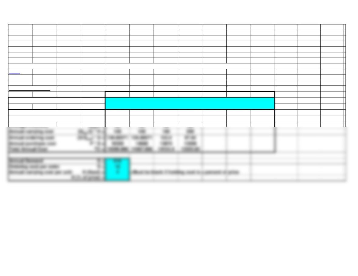
Quantity Discounts
Price Level: 1 2 3 4 5 6 7
Minimum quantity for price
Qmin = 150 80 100
Price P = 20.00 18.00 17.00 16.00
Optimal Q (for each price)
Qopt = 70 70 80 100
Number of orders per year
D/Qopt = 11.657143 11.657143 10.2 8.16
Average Inventory
Qopt/2 = 35 35 40 50
Page 11
Annual purchase cost
Total Annual Cost TC = 16599.886 14967.886 14154.4 13353.92
Annual Demand D = 816
Ordering cost per order S = 12
Annual carrying cost per unit: H (fixed) = 4 <Must be blank if holding cost is a percent of price
Quantity Discounts
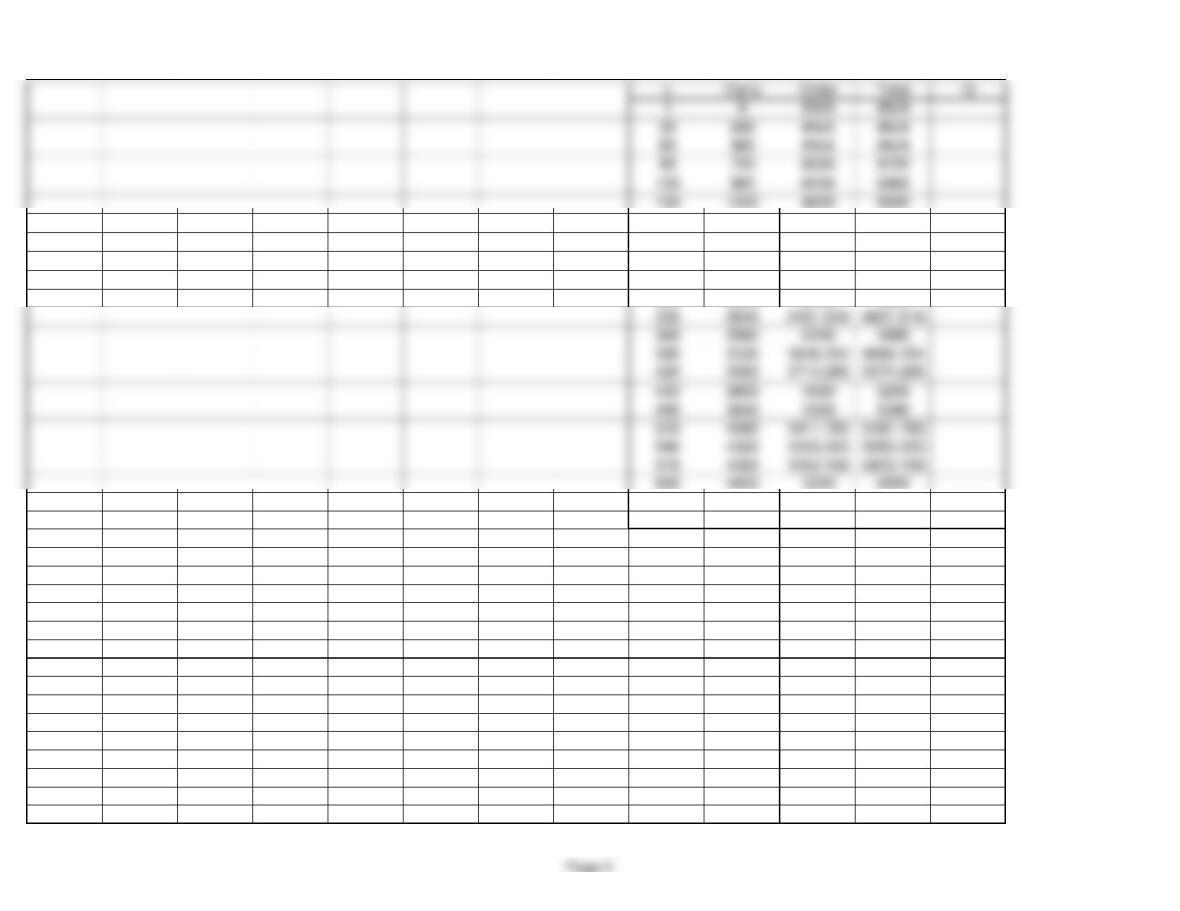
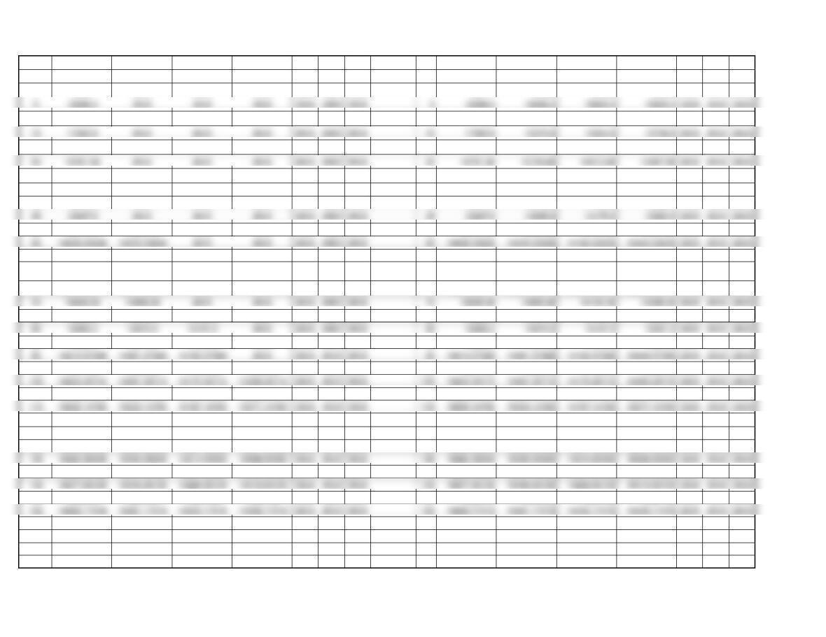
1 2 3 4 5 6 7
x 1 50 80 100 000
1 #N/A #N/A #N/A #N/A #N/A #N/A #N/A 1 26114 24482 23666 22850 #N/A #N/A #N/A
10 17319.2 #N/A #N/A #N/A #N/A #N/A #N/A 10 17319.2 15687.2 14871.2 14055.2 #N/A #N/A #N/A
20 16849.6 #N/A #N/A #N/A #N/A #N/A #N/A 20 16849.6 15217.6 14401.6 13585.6 #N/A #N/A #N/A
30 16706.4 #N/A #N/A #N/A #N/A #N/A #N/A 30 16706.4 15074.4 14258.4 13442.4 #N/A #N/A #N/A
35 16669.77143 #N/A #N/A #N/A #N/A #N/A #N/A 35 16669.77143 15037.77143 14221.77143 13405.77143 #N/A #N/A #N/A
40 16644.8 #N/A #N/A #N/A #N/A #N/A #N/A 40 16644.8 15012.8 14196.8 13380.8 #N/A #N/A #N/A
50 16615.84 14983.84 #N/A #N/A #N/A #N/A #N/A 50 16615.84 14983.84 14167.84 13351.84 #N/A #N/A #N/A
60 16603.2 14971.2 #N/A #N/A #N/A #N/A #N/A 60 16603.2 14971.2 14155.2 13339.2 #N/A #N/A #N/A
65 16600.64615 14968.64615 #N/A #N/A #N/A #N/A #N/A 65 16600.64615 14968.64615 14152.64615 13336.64615 #N/A #N/A #N/A
70 16599.88571 14967.88571 #N/A #N/A #N/A #N/A #N/A 70 16599.88571 14967.88571 14151.88571 13335.88571 #N/A #N/A #N/A
80 16602.4 14970.4 14154.4 #N/A #N/A #N/A #N/A 80 16602.4 14970.4 14154.4 13338.4 #N/A #N/A #N/A
90 16608.8 14976.8 14160.8 #N/A #N/A #N/A #N/A 90 16608.8 14976.8 14160.8 13344.8 #N/A #N/A #N/A
100 16617.92 14985.92 14169.92 13353.92 #N/A #N/A #N/A 100 16617.92 14985.92 14169.92 13353.92 #N/A #N/A #N/A
110 16629.01818 14997.01818 14181.01818 13365.01818 #N/A #N/A #N/A 110 16629.01818 14997.01818 14181.01818 13365.01818 #N/A #N/A #N/A
120 16641.6 15009.6 14193.6 13377.6 #N/A #N/A #N/A 120 16641.6 15009.6 14193.6 13377.6 #N/A #N/A #N/A
125 16648.336 15016.336 14200.336 13384.336 #N/A #N/A #N/A 125 16648.336 15016.336 14200.336 13384.336 #N/A #N/A #N/A
130 16655.32308 15023.32308 14207.32308 13391.32308 #N/A #N/A #N/A 130 16655.32308 15023.32308 14207.32308 13391.32308 #N/A #N/A #N/A
140 16669.94286 15037.94286 14221.94286 13405.94286 #N/A #N/A #N/A 140 16669.94286 15037.94286 14221.94286 13405.94286 #N/A #N/A #N/A
150 16685.28 15053.28 14237.28 13421.28 #N/A #N/A #N/A 150 16685.28 15053.28 14237.28 13421.28 #N/A #N/A #N/A
160 16701.2 15069.2 14253.2 13437.2 #N/A #N/A #N/A 160 16701.2 15069.2 14253.2 13437.2 #N/A #N/A #N/A
165 16709.34545 15077.34545 14261.34545 13445.34545 #N/A #N/A #N/A 165 16709.34545 15077.34545 14261.34545 13445.34545 #N/A #N/A #N/A
170 16717.6 15085.6 14269.6 13453.6 #N/A #N/A #N/A 170 16717.6 15085.6 14269.6 13453.6 #N/A #N/A #N/A
175 16725.95429 15093.95429 14277.95429 13461.95429 #N/A #N/A #N/A 175 16725.95429 15093.95429 14277.95429 13461.95429 #N/A #N/A #N/A
Page 12
Quantity Discounts
185 16742.92973 15110.92973 14294.92973 13478.92973 #N/A #N/A #N/A 185 16742.92973 15110.92973 14294.92973 13478.92973 #N/A #N/A #N/A
190 16751.53684 15119.53684 14303.53684 13487.53684 #N/A #N/A #N/A 190 16751.53684 15119.53684 14303.53684 13487.53684 #N/A #N/A #N/A
195 16760.21538 15128.21538 14312.21538 13496.21538 #N/A #N/A #N/A 195 16760.21538 15128.21538 14312.21538 13496.21538 #N/A #N/A #N/A
100 13353.92 100 16617.92 14888.58924 14072.65768 13256.69582
Start: 0 Stop: 200
Min Y : 0 Max Y: 24899.82857
Steps: 40 Step: 5
Page 13
ROP
Reorder Point (ROP) with EOQ Ordering Basic
<Back 14 #NUM!
14 #NUM!
Average demand d = 2 14 #NUM!
Std dev demand
sd = 014 #NUM!
Stock out risk 0.6 14 #NUM!
Average demand during lead time dLT = 14 14 #NUM!
Std dev demand during lead time
sdLT = 014 #NUM!
z = -0.253347 14 0
Safety stock SS = 0 14 1
Basic Template: You can simply copy the basic template below and paste into another worksheet.
^Top
Reorder Point (ROP) with EOQ Ordering
Average demand d = 2
Std dev demand
sd = 0
Average lead time LT = 7
Page 14
Average lead time LT = 7 14 #NUM!
Service level SL = 0.4 14 #NUM!
ROP
Stock out risk 0.6
Average demand during lead time dLT = 14
Std dev demand during lead time
sdLT = 0
Page 15
Safety stock SS = 0
Fixed Order Interval
Fixed Order Interval Model Basic
<Back
Average demand d = 30
Std dev demand
sd = 3
Lead time LT = 2
Amount on hand at reorder time A = 71
Order interval OI = 7
200
250
300
Page 16
Service level SL = 0.99
Amount to order 219.93713
Fixed Order Interval
Basic Template: You can simply copy the basic template below and paste into another worksheet.
^Top
Fixed Order Interval Model
Average demand d = 30
Std dev demand
sd = 3
Lead time LT = 2
Amount on hand at reorder time A = 71
Page 17
Stock out risk 0.01
Average demand during lead time dLT = 270
Safety stock SS = 20.937131
Single Period
Single Period Model Basic
<Back
Select demand distribution: Uniform
1
Shortage cost (revenue – cost)
Cs = 0.6 0.4
Excess cost (cost – salvage)
Ce = 0.2
Actual Stocking Level S = 450
Increment DS = 10
0.1
0.15
0.35
0.4
0.45
Uniform
Normal
Poisson
Clear
Discrete
Page 18
Minimum demand 300
Optimal Service Level
Single Period
Basic Template: You can simply copy the basic template below and paste into another worksheet.
^Top
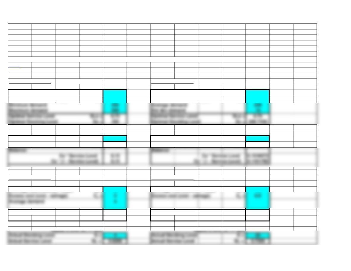
Single Period Model Demand distribution: Uniform Single Period Model Demand distribution: Normal
Shortage cost (revenue – cost)
Cs = 0.6 Shortage cost (revenue – cost) Cs = 0.6
Excess cost (cost – salvage)
Ce = 0.2 Excess cost (cost – salvage) Ce = 0.2
Actual Stocking Level S = 450 Actual Stocking Level S = 207
Actual Service Level SL = 0.7500 Actual Service Level SL = 0.7580
Single Period Model Demand distribution: Poisson Single Period Model Demand distribution: Discrete
Shortage cost (revenue – cost)
Cs = 3 Shortage cost (revenue – cost) Cs = 1.6
Ce = 2 Excess cost (cost – salvage) Ce = 0.8
Average demand 4
Optimal Service Level
SLo = 0.6
Optimal Service Level
SLo = 0.6666667
Page 19
Minimum demand 300 Average demand 200
Maximum demand 500 Std dev demand 10
Optimal Service Level
SLo = 0.75
Optimal Service Level
Optimal Stocking Level So = 450 Optimal Stocking Level So = 206.7449
Single Period
Balance: Balance:
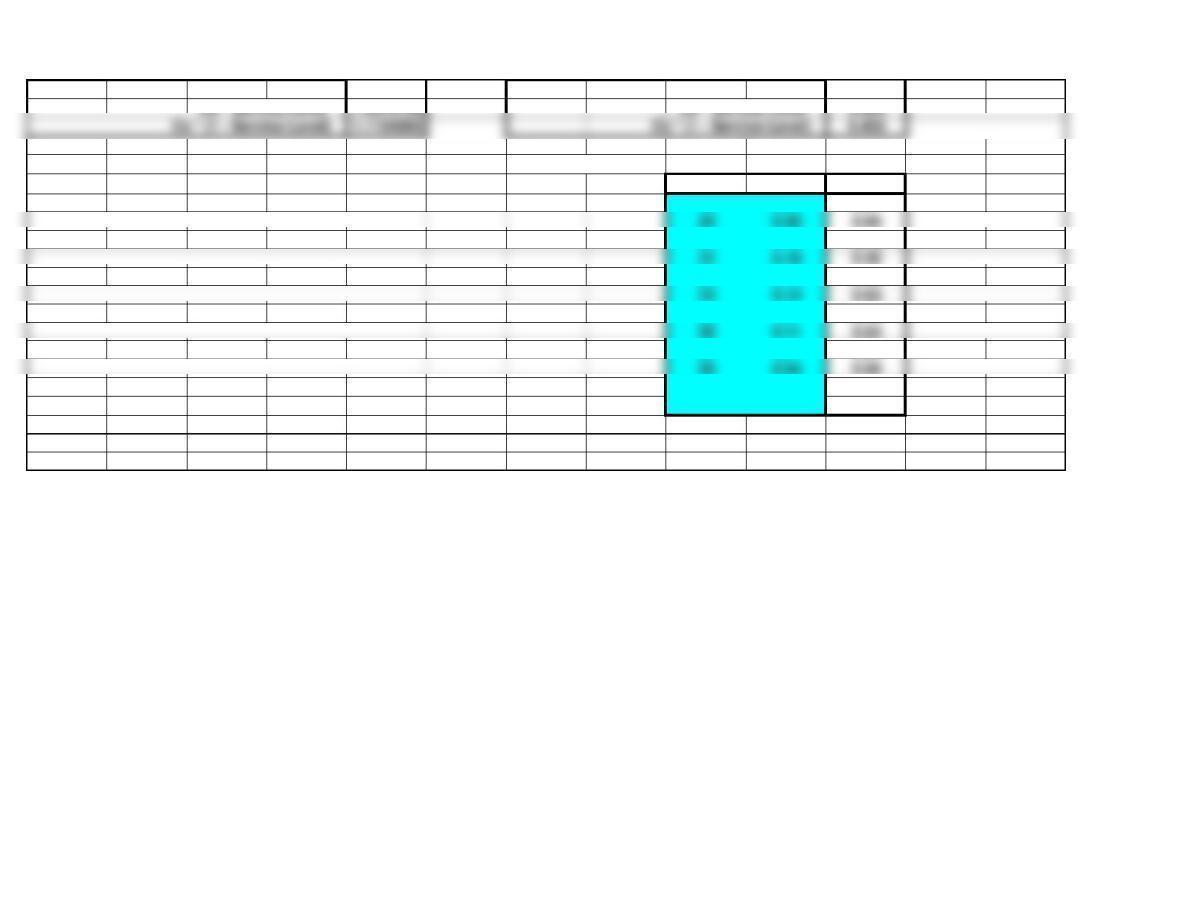
Discrete Distribution:
Demand Freq Cum
19 0.01 0.01
20 0.05 0.06
21 0.12 0.18
22 0.18 0.36
23 0.13 0.49
24 0.14 0.63
25 0.1 0.73
26 0.11 0.84
27 0.1 0.94
28 0.04 0.98
29 0.02 1
1
Page 20