Chapter 13 – Inventory Management
13-1
CHAPTER 13
INVENTORY MANAGEMENT
Teaching Notes
This is a fairly long and important chapter. Important points are:
2. The key issues are when to order and how much to order.
4. EOQ models answer the question of how much to order. Variations of the basic EOQ model
include the quantity discount model and the economic run size model.
6. ROP models are used to answer the question of when to order. Different models are used,
depending on whether demand, lead time, or both are variable.
8. All of the models in this chapter pertain to independent demand.
The Single-Period Model is used to handle ordering of perishables (such as fresh fruits and vegetables,
seafood, and cut flowers) as well as items that have a limited useful life (such as newspapers and
Answers to Discussion and Review Questions
1. Inventories are held (1) to take advantage of price discounts, (2) to take advantage of economic
2. Effective inventory management requires (1) cost information, information on demand and lead
time (amounts and variabilities), an accounting system, and a priority system (e.g., A-B-C).
3. Carrying or holding costs include interest, security, warehousing, obsolescence, and so on.
Procurement costs relate to determining how much is needed, vendor analysis, inspection of
Chapter 13 – Inventory Management
13-2
4. The RFID (Radio Frequency Identification) chip tags are beginning to be used with consumer
products and they contain bits of data, such as product serial number. Scanners will automatically
read the information on an RFID chip into a database, so the companies can keep track of sales
5. It may be inappropriate to compare the inventory turnover ratios of companies in different
industries because the production process, requirements and the length of production run varies
6. a. Only one product is involved.
b. Annual demand requirements are known.
7. The total cost curve is relatively flat in the vicinity of the EOQ, so that there is a “zone” of values
8. As the carrying cost increases, holding inventory becomes more expensive. Therefore, in order to
9. Safety stock is inventory held in excess of expected demand to reduce the risk of stockout
presented by variability in either lead time or demand rates.
10. Safety stock is large when large variations in lead time and/or usage are present. Conversely,
11. Service level can be defined in a number of ways. The text focuses mainly on “the probability
that demand will not exceed the amount on hand.” Other definitions relate to the percentage of
Chapter 13 – Inventory Management
13-3
12. The A-B-C approach refers to the classification of items stocked according to some measure of
13. In effect, this situation is a “quantity discount” case with a time dimension. Hence, buying larger
quantities will result in lower annual purchase costs, lower ordering costs (fewer orders), but
14. Annual carrying costs are determined by average inventory. Hence, a decrease in average
15. The Single-Period Model is used when inventory items have a limited useful life (i.e., items are
not carried over from one period to the next).
17. A company can reduce the need for inventories by:
a. using standardized parts
b. improved forecasting of demand
c. using preventive maintenance on equipment and machines
Taking Stock
1. a. If we buy additional amounts of a particular good to take advantage of quantity discounts,
then we will save money on a per unit purchasing cost of the item. We will also save on
ordering cost because since we bought a larger quantity, we will not have to order this item as
frequently. However, as a result of ordering larger quantity, we will have to carry larger
inventory in stock, which in turn will result in an increase in inventory holding cost.
Chapter 13 – Inventory Management
13-4
2. In making inventory decisions involving holding costs, setting inventory levels and deciding on
quantity discount purchases, the materials manager, plant manager, production planning and
3. The technology has had a tremendous impact on inventory management. The utilization of bar
coding has not only reduced the cost of taking physical inventory but also enabled real time
Critical Thinking Exercise
1. Including a wider range of foods provide fast food companies with a competitive edge in terms of
improving customer satisfaction and service. However, it has also complicated the operational
function of the company. Expansion of menu offerings can create problems for inventory
2. a. How important is the item? For example, does it relate to a holiday or other important event,
such as graduation cards?
3. Among considerations are:
How many stamps does he now have? Does he know how many he has? If so, how many?
What is his usage rate or current need for stamps?
What else does he need the cash for today?
Can he get more money at a bank or ATM?
Chapter 13 – Inventory Management
13-5
Can he purchase “forever stamps” and temporarily avoid a price increase?
4. Student answers will vary.
Memo Writing Exercises
1. Cost of carrying inventory must be weighted against the following costs:
a. cost of shortages (finished goods inventory)
2. The possible advantages of using a single supplier include:
a. obtaining a discount due to additional volume purchased from the supplier
b. building trust and working with the supplier so that the material will be delivered in a timely
fashion to avoid stockouts and excess inventory.
The possible advantages of using multiple suppliers include:
a. the adverse effect of tardiness will be felt much less when there are multiple sources for the
materials.
Chapter 13 – Inventory Management
13-6
Solutions
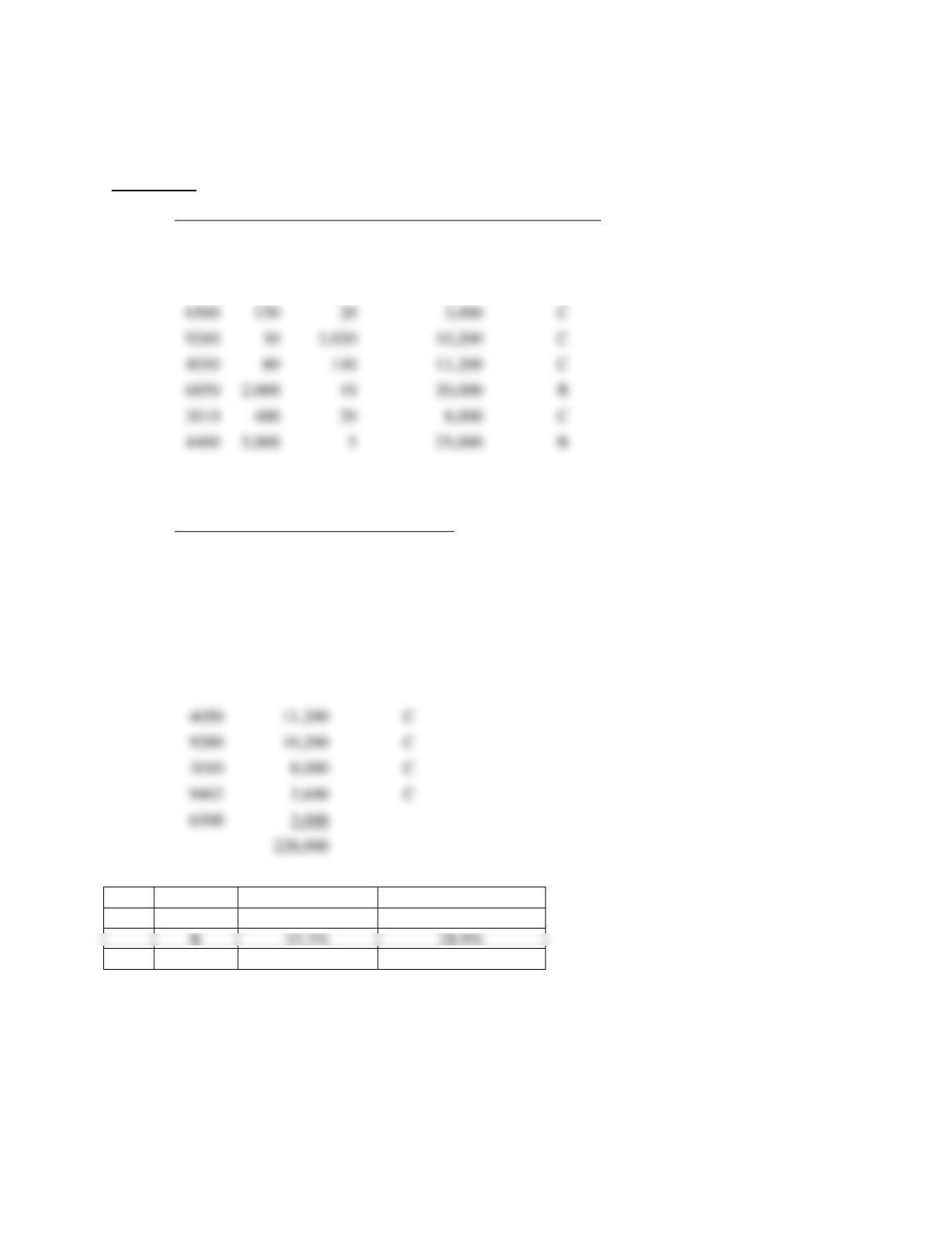
1. a.
Item
Usage
Unit Cost
Usage x Unit Cost
Category
4021
90
$1,400
$126,000
A
9402
300
12
3,600
C
4066
30
700
21,000
B
In descending order:
Item
Usage x Cost
Category
4021
$126,000
A
4400
25,000
B
4066
21,000
B
6850
20,000
B
11,200
C
9280
10,200
C
3010
8,000
C
9402
3,600
C
6500
1. b.
Category
Percent of Items
Percent of Total Cost
A
11.1%
55.3%
C
55.6%
15.8%
9280
10
10,200
C
4050
80
140
11,200
C
6850
2,000
10
20,000
B
4400
5,000
25,000
B
Chapter 13 – Inventory Management
13-7
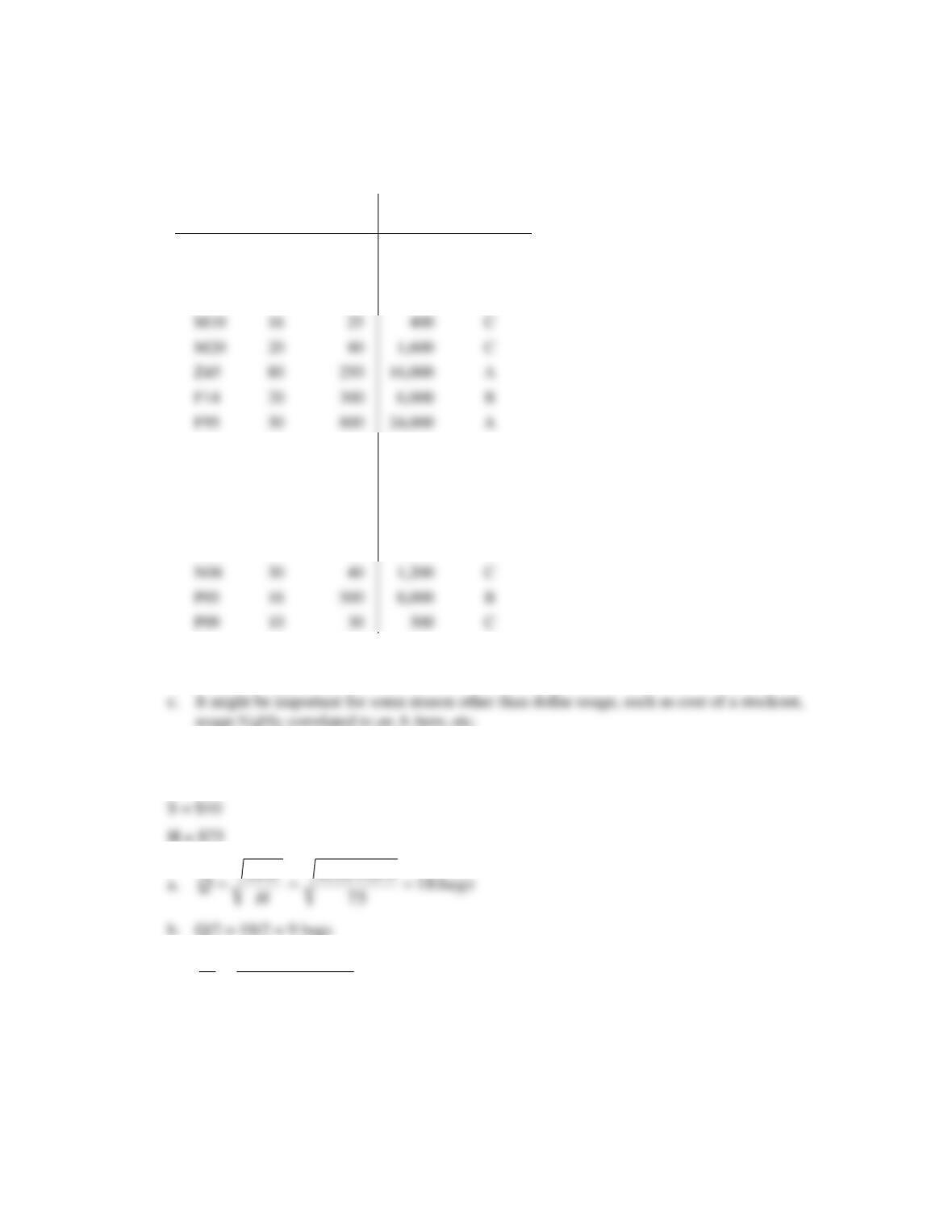
2. The following table contains figures on the monthly volume and unit costs for a random sample
of 16 items for a list of 2,000 inventory items.
Dollar
Item
Unit Cost
Usage
Usage
Category
K34
10
200
2,000
C
K35
25
600
15,000
A
K36
36
150
5,400
B
F99
20
60
1,200
C
D45
10
550
5,500
B
D48
12
90
1,080
C
D52
15
110
1,650
C
D57
40
120
4,800
B
N08
30
40
1,200
C
P09
10
30
300
C
a. Develop an A-B-C classification for these items. [See table.]
b. How could the manager use this information? To allocate control efforts.
3. D = 1,215 bags/yr.
c.
orders
ordersbags
bags
Q
D 5.67
/ 18
215,1 ==
M10
16
25
400
C
M20
20
80
1,600
C
F14
20
300
6,000
B
F95
30
800
24,000
A
Chapter 13 – Inventory Management
13-8
d.
S
Q
D
H2/QTC +=
350,1$675675)10(
18
215,1
)75(
2
18 =+=+=
4. D = 40/day x 260 days/yr. = 10,400 packages
S = $60 H = $30
a.
oxesb 20496.203
30
60)400,10(2
H
DS2
Q0====
Chapter 13 – Inventory Management
13-9
5. D = 750 pots/mo. x 12 mo./yr. = 9,000 pots/yr.
Price = $2/pot S = $20 H = ($2)(.30) = $.60/unit/year
60.
H
6.774
2
TC = 232.35 + 232.36
= 464.71
If Q = 1500
6. u = 800/month, so D = 12(800) = 9,600 crates/yr.
H = .35P = .35($10) = $3.50/crate per yr.
50.3$
H
TC at EOQ:
.71.371,1$)28(
392
600,9
)50.3(
2
392 =+
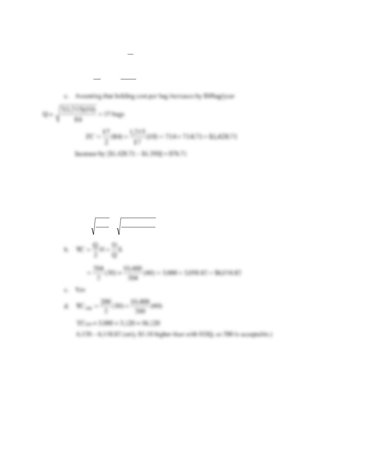
Savings approx. $364.28 per year.
Chapter 13 – Inventory Management
13-10
7. H = $2/month
a.
16.74
2
55)100(2
Q:D
H
DS2
Q010 ===
83.90
55)150(2
Q:D 02 ==
1–6 TC74 = $148.32
*140$)45(
100
)2(
50
TC
=+=
7–12 TC91 = $181.66
185$)45(
150
)2(
50
TC
=+=
Chapter 13 – Inventory Management
13-11
8. D = 27,000 jars/month
a.
.243,464.242,4
18.
60)000,27(2
H
DS2
Q===
TC=
S
D
H
Q+
32.1$
TC4000 =
765)60(
000,4
000,27
)18(.
2
000,4 =
+
TC4243 =
68.76360
243,4
000,27
)18(.
2
243,4 =
+
b. Current:
75.6
000,4
000,27
Q
D==
Difference
Chapter 13 – Inventory Management
13-12
9. p = 5,000 hotdogs/day
a.
4,812] to[round 27.812,4
750,4
000,5
45.
66)000,75(2
up
p
H
DS2
Q0==
−
=
10. p = 50/ton/day
u = 20 tons/day
a.
bags] [10,328 tons 40.516
2050
50
5
100)000,4(2
up
p
H
DS2
Q0=
−
=
−
=
b.
]bags 8.196,6 .approx[ tons 84.309)30(
4.516
)up(
Q
Imax ==−=
c. Run length =
days 33.10
50
4.516
P
Q==
e. Q = 258.2
D= 20 tons/day x 200 days/yr. = 4,000 tons/yr.
Chapter 13 – Inventory Management
11. S = $300
D = 20,000 (250 x 80 = 20,000)
a.
=
−
=
−
=80200
200
10
300)000,20(2
up
p
H
DS2
Q0
Q0 = (1,095.451) (1.2910) = 1,414 units
b. Run length =
days 07.7
200
414,1
P
Q==
No, because present demand could not be met.
e. 1) Try to shorten setup time by .40 days.
f. In order to be able to accommodate a job of 10 days, plus one day for setup, there would
need to be an11 day supply at Imax, which would be 880 units on hand. Solving the
following for Q, we find:
units 880)80200(
200
)(
max =−=−= Q
up
P
Q
I
Q = 1,467.
Chapter 13 – Inventory Management
13-14
12. p = 800 units per day
d = 300 units per day
Q0 = 2000 units per day
a. Number of batches of heating elements per year =
5.37
000,2
000,75 =
batches per year
c. Maximum inventory or Imax can be found using the following equation:
units 625
2
2501
2
inventory Average
units 250125)(2,000)(.6
800
300800
0002
0
===
==
−
=
−
=
,
I
,,
p
dp
QI
max
max
Chapter 13 – Inventory Management
13-15
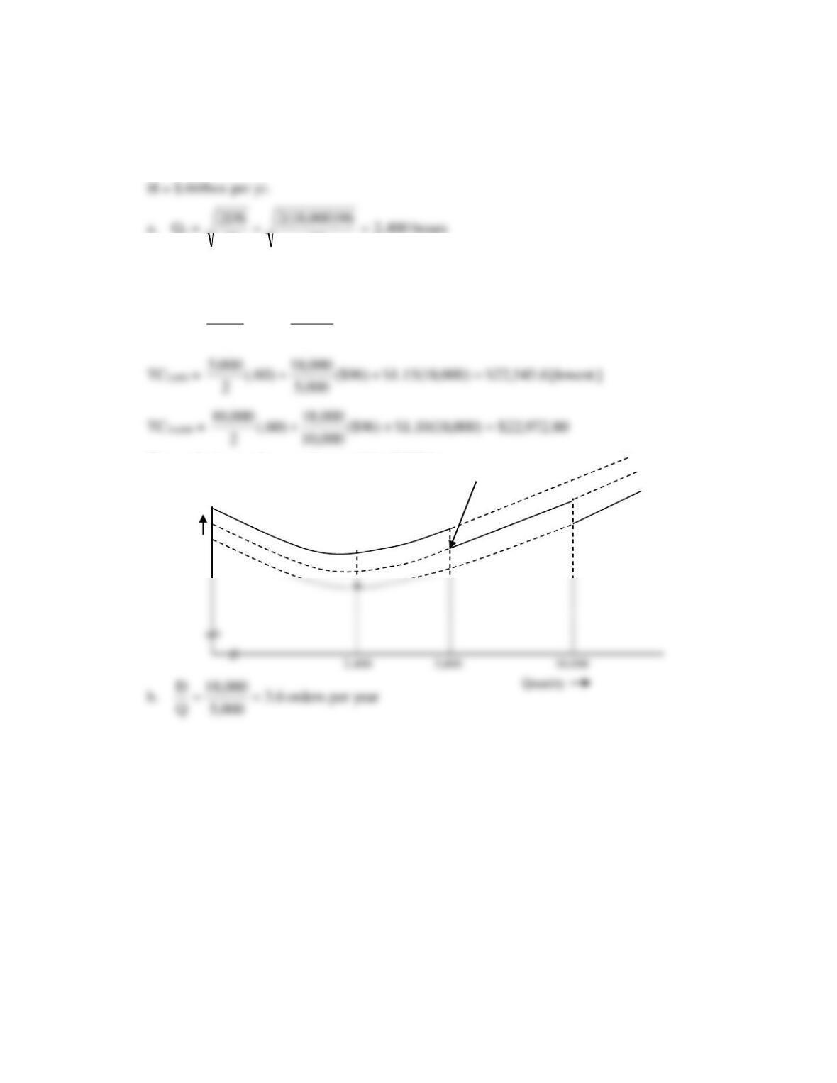
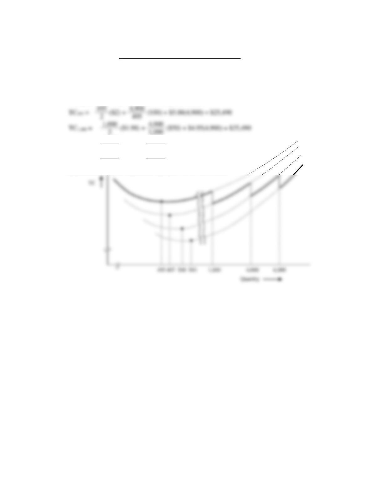
13. D = 18,000 boxes/yr.
S = $96
60.
H
Since this quantity is feasible in the range 2000 to 4,999, its total cost and the total cost of all
lower price breaks (i.e., 5,000 and 10,000) must be compared to see which is lowest.
TC2,400 =
040,23$)000,18(20.1$)96($
400,2
000,18
)60(.
2
400,2 =++
Hence, the best order quantity would be 5,000 boxes.
•
TC
•
•
Lowest TC
Chapter 13 – Inventory Management
13-16
14.
a.
S = $48
D = 25 stones/day x 200 days/yr. = 5,000 stones/yr.
Quantity
Unit Price
a.
H = $2
1 – 399
$10
400 – 599
9
90.489
2
48)000,5(2
H
DS2
Q===
600 +
8
b.
H = .30P
(Feasible)
Q
D
Q
422
600
$8/stone)at feasibleNot (
NF 447
)8(30.
48)000,5(2
EOQ
8$
==
Since an order quantity of 600 would have a lower cost than 422, 600 stones is
the optimum order size.
c.
ROP = 25 stones/day (6 days) = 150 stones.
TC
Chapter 13 – Inventory Management
13-17
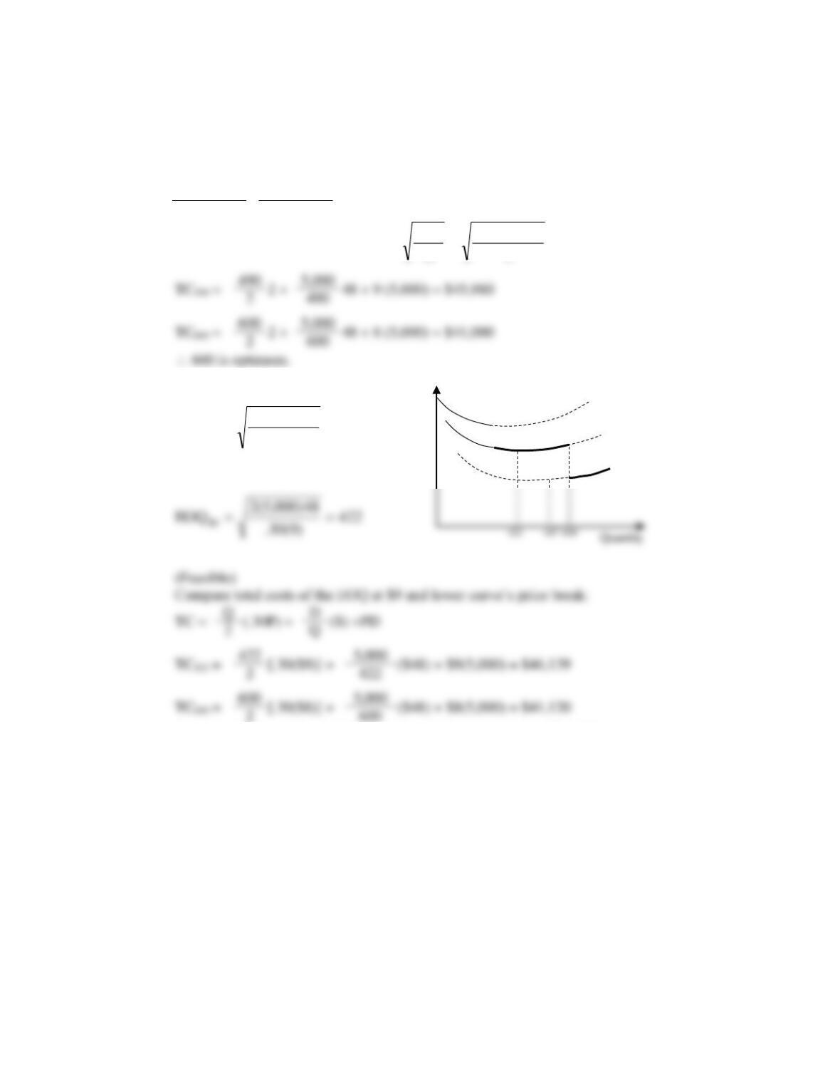
15.
Range
P
H
Q
D = 4,900 seats/yr.
0–999
$5.00
$2.00
495
H = .4P
1,000–3,999
4.95
1.98
497 NF
S = $50
4,000–5,999
4.90
1.96
500 NF
6,000+
4.85
1.94
503 NF
Compare TC495 with TC for all lower price breaks:
TC4,000 =
4,000
($1.96) +
4,900
($50) + $4.90(4,900) = $27,991
2
4,000
TC6,000 =
6,000
($1.94) +
4,900
($50) + $4.85(4,900) = $29,626
2
6,000
Hence, one would be indifferent between 495 or 1,000 units
TC495 =
($2) +
4,900
($50) + $5.00(4,900) = $25,490
2
TC1,000 =
1,000
($1.98) +
4,900
($50) + $4.95(4,900) = $25,490
2
1,000
Chapter 13 – Inventory Management
13-18
16. D = (800) x (12) = 9600 units
S = $40
H = (25%) x P
For Supplier A:
)]600,9)(6.13[()40(
500
600,9
)6.13)(25(.
2
500
TC
75.107,134$TC
500
81.471
81.471
++
=
=
For Supplier B:
85.141,133$TC
520,13192.81093.810TC
53.473
2
)7.13)(25(.
81.471
81.471
=
++=
Chapter 13 – Inventory Management
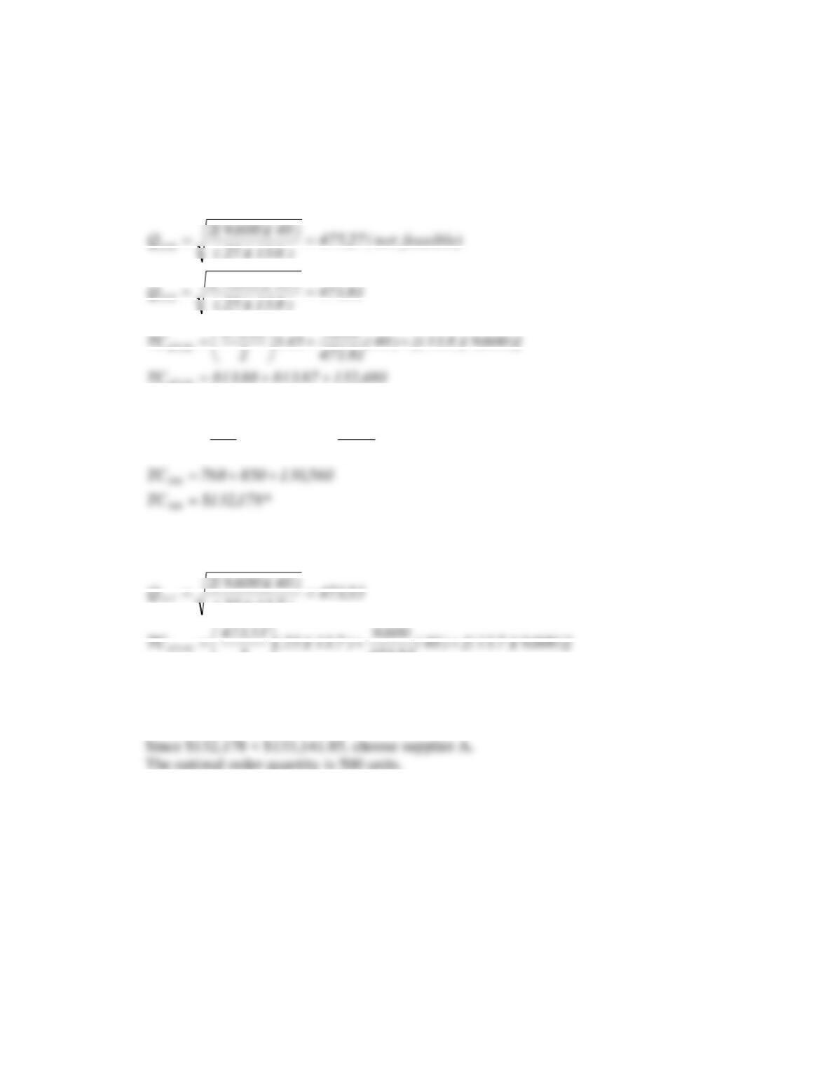
13-19
17. D = 3600 boxes per year
Q = 800 boxes (recommended)
S = $80 /order
H = $10 /order
Even though the inventory total cost curve is fairly flat around its minimum, when there are
quantity discounts, there are multiple U shaped total inventory cost curves for each unit price
depending on the unit price. Therefore when the quantity changes from 800 to 801, we shift to a
different total cost curve.
The order quantity of 801 is preferred to order quantity of 800 because TCQ=801 < TCQ=800 or
7964.55 < 8320.
)D*P(S
Q
D
H
2
Q
TC
boxes 240
10
)80)(600,3(2
H
DS2
EOQ
EOQ
+
+
=
===
Chapter 13 – Inventory Management
13-20
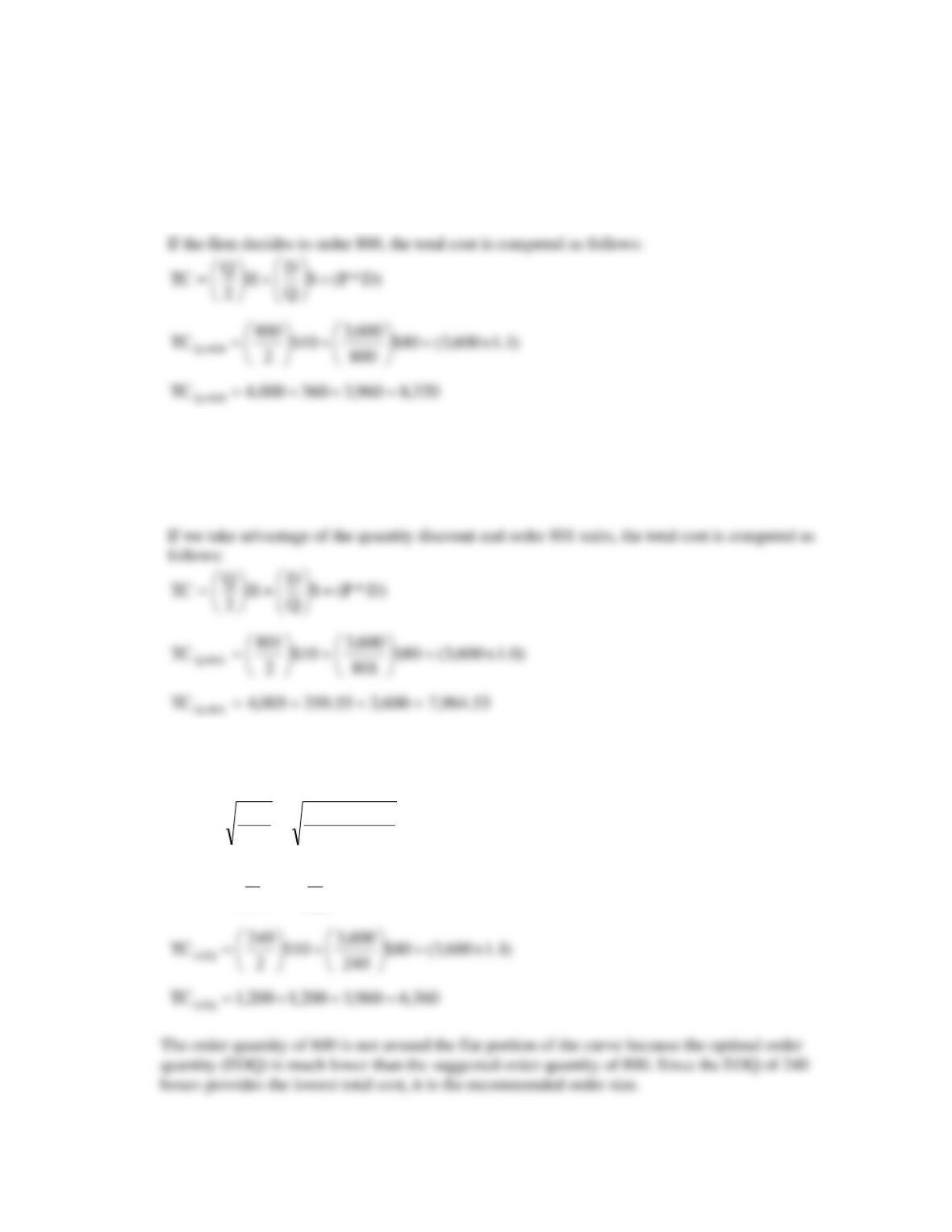
18. Daily usage = 800 ft./day Lead time = 6 days
Service level desired: 95 percent. Hence, risk should be 1.00 – .95 = .05
19. Expected demand during LT = 300 units
dLT = 30 units
20. LT demand = 600 lb.
d LT = 52 lb.
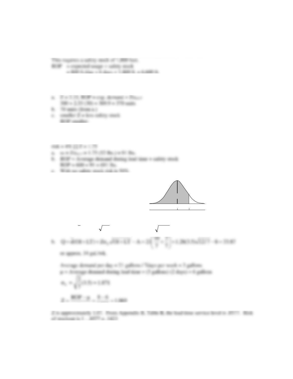
21. −
d = 21 gal./wk.
d = 3.5 gal./wk.
LT = 2 days
SL = 90 percent requires z = +1.28
a.
gallons 398(3.5)(2/7)281(2/7)21)(LTz(LT)dROP d.. =+=+=
871.1
L
6 8.39 gallons
0 1.28 z-scale
90%