13-38 CHAPTER 13: ADDITIONAL INTEGRATION TOPICS
76. C‘(x) = 65 20
10.4
x
x
, C(0) = 11,000
x
10.4
x
dx
x
0.4
0.16
Since C(0) = 11,000, we have C1 = 11,000 and therefore,
C(x) = 50x + 37.5 ln(1 + 0.4x) + 11,000
0
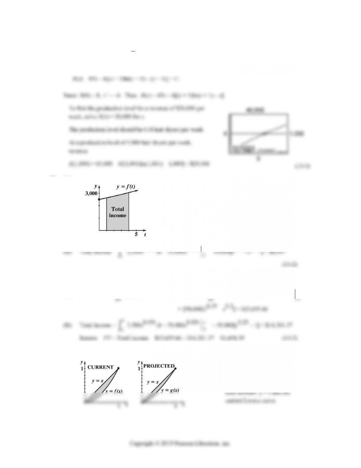
78. FV = erT
0
T
f(t)e-rt dt
te–0.037t dt =
0.037
0.037
t
te
– 1
0.037
e–0.037t dt =
0.037
0.037
t
te
+ 1
0.037
0.037
0.037
t
e
+ C
0.037
0.037
t
te
–
0.0.37
2
0.037
t
e
Thus,
FV =
5
0.037 0.037
0.185
2
0
200 0.037 0.037
tt
te e
e
0.037 5 0.037 0
0.037 5 0.037 0
0.185
50
ee
ee
22
EXERCISE 13-4 13-39
Copyright © 2019 Pearson Education, Inc.
=
0.185 0.185 0.185 0.185 0.185
22
1000 200 200
0.037 0.037 0.037
eee
=
0 0 0.185
22
1000 200 200
0.037 0.037 0.037
eee
=
0.185
2
1000 0.037 200 200 $2,661.57
0.037
e
5
5
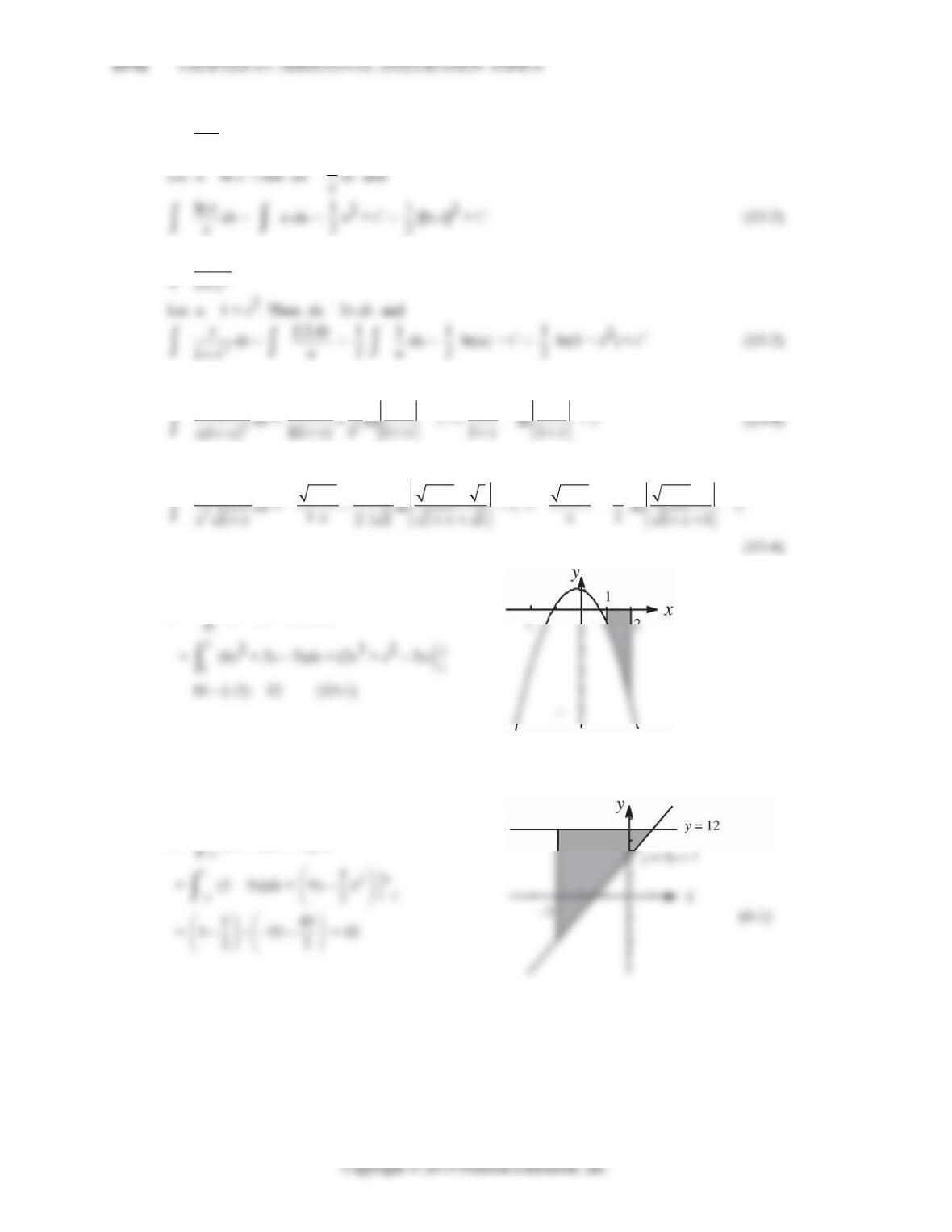
80. Index of Income Concentration:
2
1
0
[x – f(x)]dx = 2
1
0
2
113
2
x
xx
dx = 2
1
0
x dx –
1
0
x213
x
dx
For the second integral, use Formula 23 with a = 1 and b = 3:
1
1
2
3
2(135 36 8) (1 3 )
xx x
82.
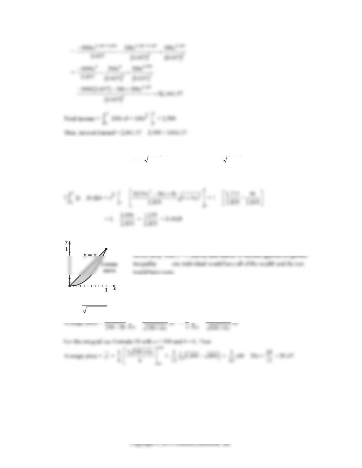
As the area bounded by the two curves gets larger, the Lorenz curve
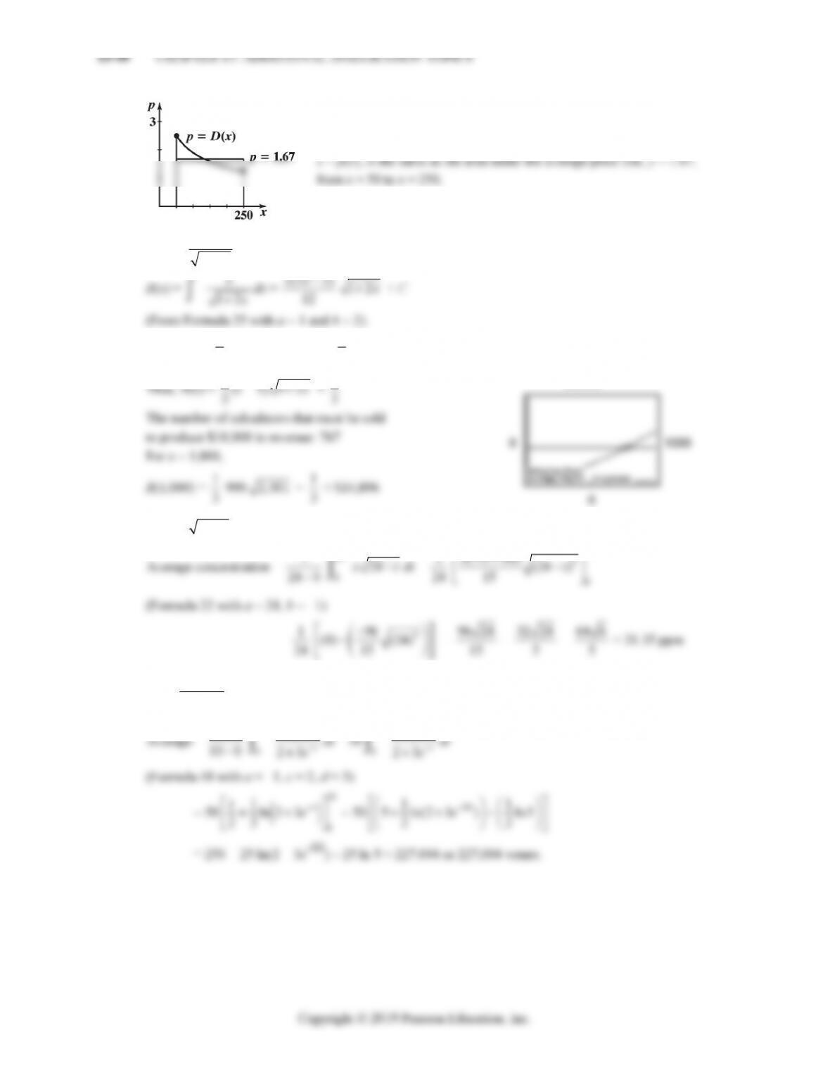
84. D(x) = 50
100 6
x
x
x
250
50
250
1
50
CHAPTER 13 REVIEW 13-43
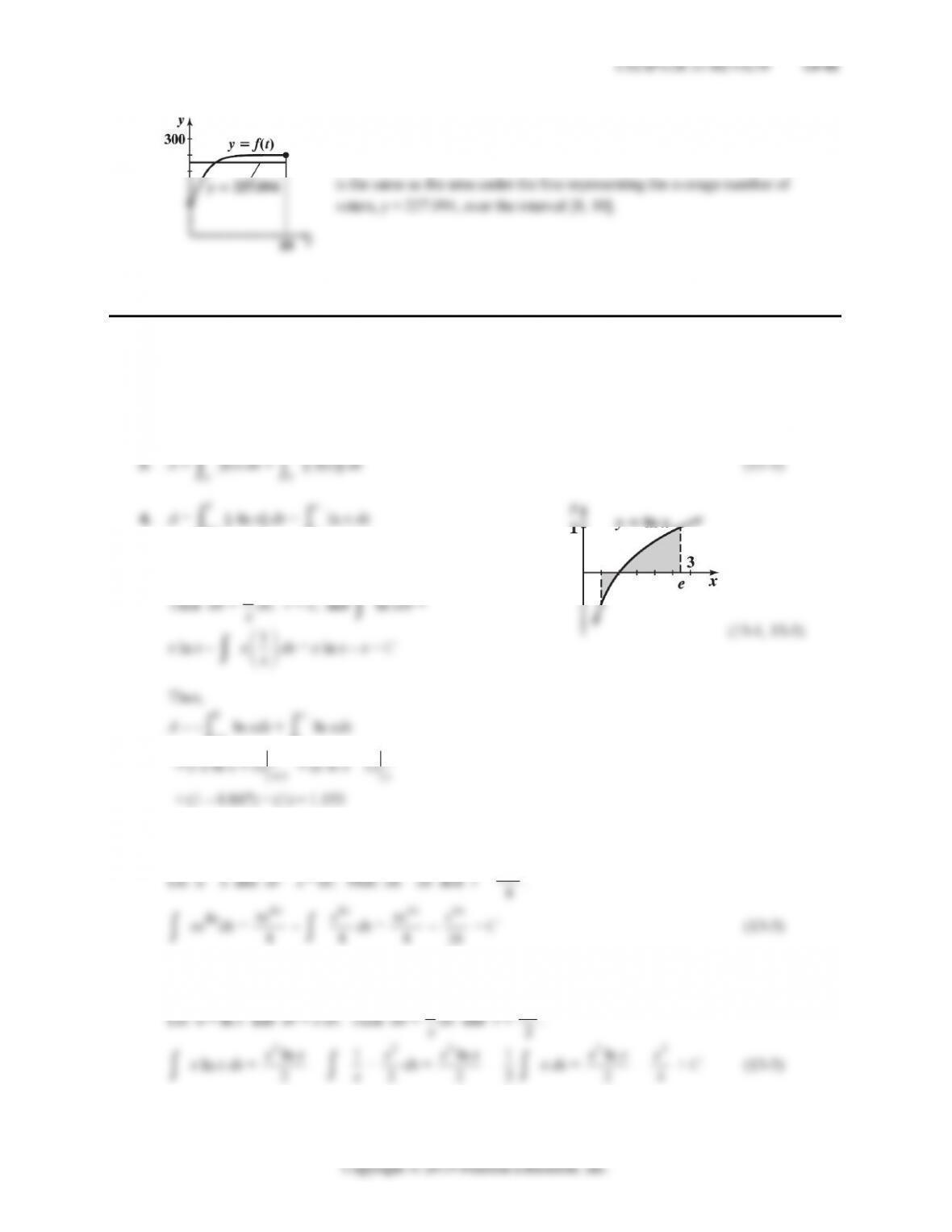
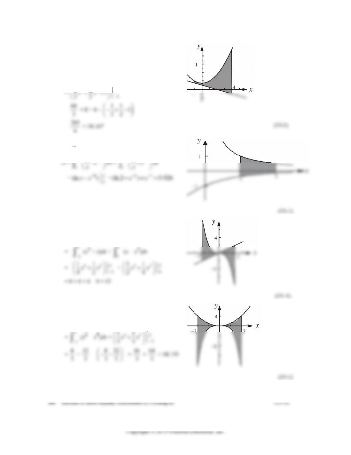
13. y = –x + 2; y = x2 + 3 on [–1, 4]
A =
4
1
[(x2 + 3) – (–x + 2)] dx
=
4
1
(x2 + x + 1) dx
x
11
4
6 ≈ 34.167
14. y = 1
x
; y = − e–x on [1, 2]
2
1
x
2
1
x
15. y = x; y = –x3 on [–2, 2]
A =
0
2
(–x3 – x)dx +
2
0
x – (–x3)dx
0
2
x
x
16. y = x2; y = –x4 on [–2, 2]
A =
2
2
[x2 – (–x4)]dx
x
2
11
2
17. Income is more equally distributed in Venezuela. (13-1)
13-44 CHAPTER 13: ADDITIONAL INTEGRATION TOPICS
b
a
20. A =
c
b
[g(x) – f(x)]dx (13-1)
c
d
22. A =
b
a
[f(x) – g(x)]dx +
c
b
[g(x) – f(x)]dx +
d
c
[f(x) – g(x)] dx (13-1)
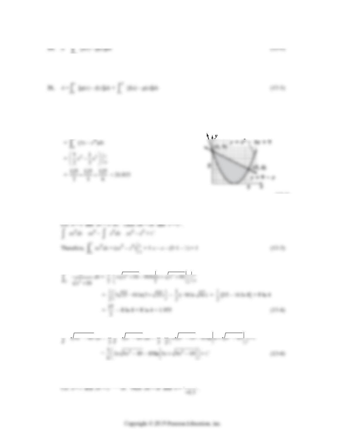
23. A =
5
0
[(9 – x) – (x2 – 6x + 9)]dx
5
23 6
(13-1)
24.
1
0
xexdx. Use integration-by-parts.
25. Use Formula 38 with a = 4
3
2
x
116 16ln 16
3
26. Let u = 3x, then du = 3 dx. Now, use Formula 40 with a = 7.
2
249udu = 1
149 49ln 49
Copyright © 2019 Pearson Education, Inc.
28.
x2 ln x dx. Use integration-by-parts.
x
3
x
x
x
x
x
x
x
29. Use Formula 48 with a = 1, c = 1, and d = 2.
12
x
edx = 1
111
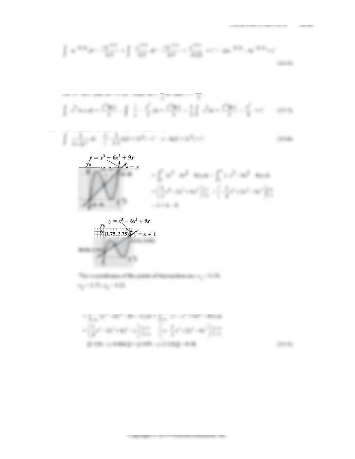
30. (A)
A
=
2
0
[(x3 – 6x2 + 9x) – x] dx +
4
2
[x – (x3 – 6x2 + 9x)] dx
2
4
x
x
(B)
A = 1.75
0.14
[(x3 – 6x2 + 9x) – (x + 1)] dx + 4.11
1.75
[(x + 1) – (x3 – 6x2 + 9x)] dx
x
x
13-46 CHAPTER 13: ADDITIONAL INTEGRATION TOPICS
31. 22
3
0
;() .
x
x
edxfx e
Partition [0,3] into three equal subintervals: 0123
0, 1, 2, 3, 1.xxxx x
x
()
f
x
1 2.7183
3 8103.0839
(13-4)
32. 22
3
;() .
x
x
edxfx e
Partition [0,3] into five equal subintervals:
x
()
f
x
0.6 1.4333
1.8 25.5337
3 8103.0839
33.
5
22
(ln ) , ( ) (ln ) .
x
dx f x x
Partition [1,5] into four equal subintervals:
x
()
f
x
1 0
2 0.4805
4 1.9218
CHAPTER 13 REVIEW 13-47
Copyright © 2019 Pearson Education, Inc.
4[(1) 4(2) 2(3) 4(4) (5)](1/3)Sf f f f f
[0 1.9220 2.4138 7.6872 2.5903](1/ 3) 4.87 (13-4)
34.
5
22
(ln ) , ( ) (ln ) .
x
dx f x x
Partition [1,5] into eight equal subintervals:
x
()
f
x
1 0
2 0.4805
3 1.2069
4 1.9218
5 2.5903
(13-4)
35.
2
(ln )
x
x
dx =
u2du =
3
3
u + C =
3
(ln )
3
x
+ C
x
36. x(ln x)2dx. Use integration-by-parts.
Let u = (ln x)2 and dv = x dx. Then du = 2(ln x)1
x
dx and v =
2
2
x
.
22
x
x
2
22
2
24
2
2
4
13-48 CHAPTER 13: ADDITIONAL INTEGRATION TOPICS
37. Let u = x2 – 36. Then du = 2xdx.
236
x
xdx =
212
( 36)
x
xdx = 1
2
12
1
udu = 1
2
u–1/2du
= 1
2 ·
12
12
u + C = u1/2 + C = 236x + C (13-2)
38. Let u = x2, du = 2xdx.
Then use Formula 43 with a = 6.
x
xdx = 1
du
u = 1
+ C = 1
36xx
+ C (13-4)
39.
4
0
x ln(10 – x)dx
Consider
x ln(10 – x)dx =
(10 – t)ln t (–dt) =
t ln t dt – 10
ln t dt.
Substitution: 10 , , 10txdtdxxt
Let u = ln t, dv = t dt. Then du = 1
tdt, v =
2
t ln t dt = t ln t –
t · 1
tdt = t ln t – t + C
Thus,
x
4
22
24
40. Use Formula 52 with n = 2.
(ln x)2dx = x(ln x)2 – 2
ln x dx
x
x
13-50 CHAPTER 13: ADDITIONAL INTEGRATION TOPICS
ln z dz = z ln z –
z1
z
dz = z ln z –
dz = z ln z – z + C
Therefore,
ln(x + 1)dx = (x + 1)ln(x + 1) – (x + 1) + C and
47. (A)
4
48. f(t) = 2,500e0.05t, r = 0.04, T = 5
(A) FV = e(0.04)5
5
2,500e0.05t e–0.04t dt = 2,500e0.2 5
e0.01t dt = 250,000e0.2 e0.01t 5
CHAPTER 13 REVIEW 13-51
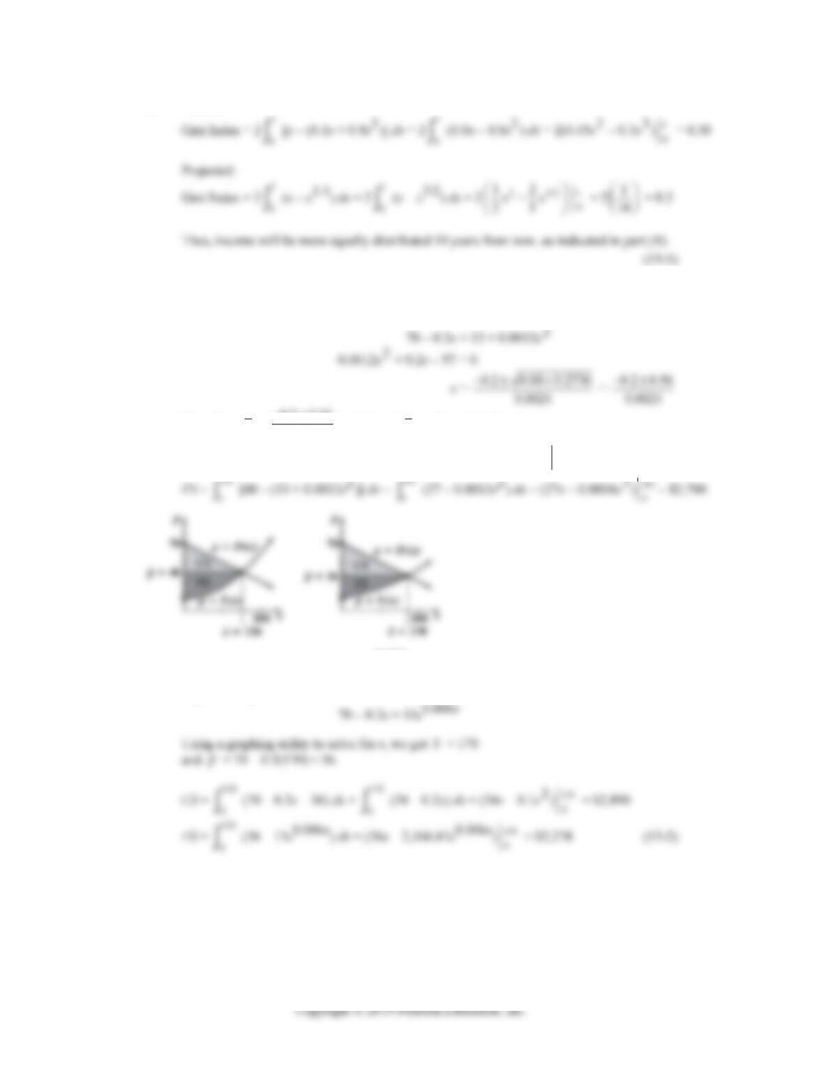
(C) Current:
1
1
50. (A) p = D(x) = 70 – 0.2x, p = S(x) = 13 + 0.0012x2
Equilibrium price: D(x) = S(x)
x = 0.2 0.04 0.2736
0.0024
0.0024
Therefore,
x
= 0.2 0.56
0.0024
= 150, and p = 70 – 0.2(150) = 40.
CS = 150
0
(70 – 0.2x – 40) dx = 150
0
(30 – 0.2x) dx = (30x – 0.1x2)150
0= $2,250
(B) p = D(x) = 70 – 0.2x, p = S(x) = 13e0.006x
Equilibrium price: D(x) = S(x)
x
13-52 CHAPTER 13: ADDITIONAL INTEGRATION TOPICS
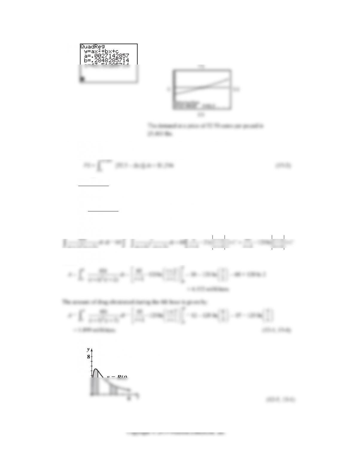
51. (A) Graph the quadratic regression model and the line p = 52.50
to find the point of intersection.
(B) Let S(x) be the quadratic regression model found in part (A). Then the producers’ surplus at the
price level of 52.5 cents per pound is given by
25.403
52. R(t) = 2
60
(1)( 2)
t
tt
The amount of the drug eliminated during the first hour is given by
A =
1
0
2
60
(1)( 2)
t
tt
dt
First use Formula 19 with a = 1, b = 1, c = 2, d = 1 to find the indefinite integral:
(1)(2)
tt
11 1 1
(1)(2)
tt t t
tt
Now,
1
60
t
1
60 2
t
53.
CHAPTER 13 REVIEW 13-53
54. f(t) = 2
43 03
(1)
0otherwise
t
t
1
43
2
(1)tdt = 4
3
u–2du =
31
= – 4
3u + C = 4
3( 1)t
+ C
1
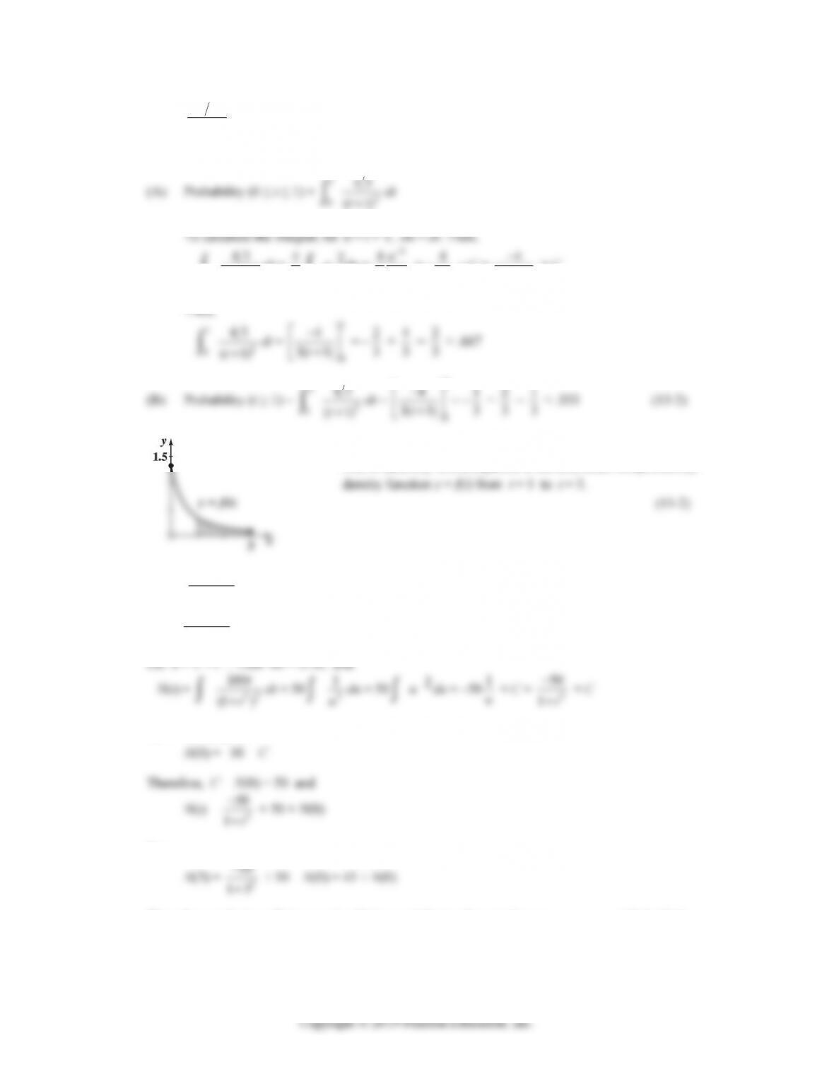
55.
The probability that the doctor will spend more than an hour
with a randomly selected patient is the area under the probability
56. N‘(t) = 22
100
(1 )
t
t. To find N(t), we calculate
22
100
(1 )
t
tdt
Let u = 1 + t2. Then du = 2t dt, and
100
t
1
50
At t = 0, we have
Now,
50
Thus, the population will increase by 45 thousand during the next 3 years. (12-5, 13-1)
13-54 CHAPTER 13: ADDITIONAL INTEGRATION TOPICS
57. We want to find Probability (t ≥ 2) =
2
()
f
tdt
Since
f(t) dt =
2
f(t) dt +
2
f(t) dt = 1,
2
2