13-1
13 ADDITIONAL INTEGRATION TOPICS
EXERCISE 13-1
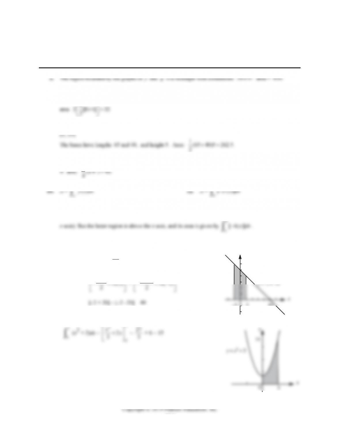
4. The region bounded by the graphs of f and g is a parallelogram with vertices (0,0), (8,4), (8,0),
(0, – 4). The x-axis divides the parallelogram into two congruent right triangles with base 8 and height 4:
2
6. The region bounded by the graphs of f and g is a trapezoid with vertices (5,90), (10,80), (10,40),
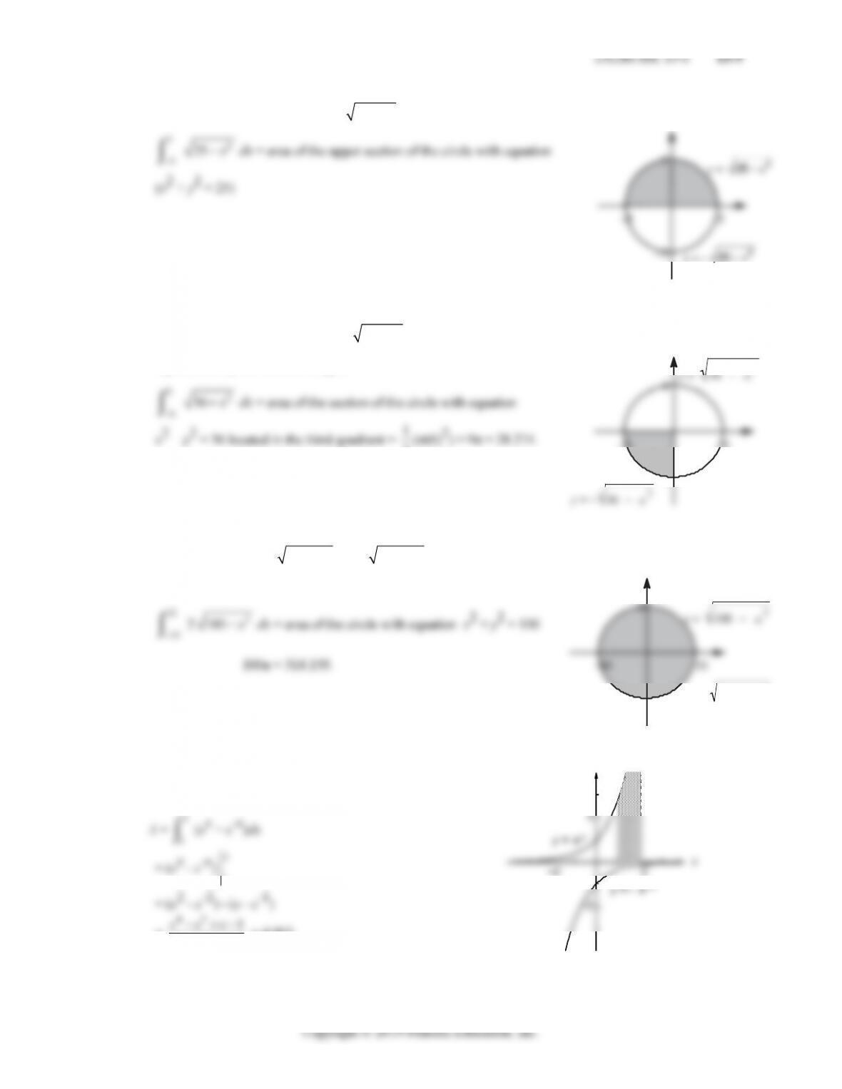
8. The region bounded by the graphs of f and g is one quarter of the disk centered at the origin with radius
1(4) 4.
a
0
14. The area of the shaded region in Figure (C) is the same as the area of the region between the curve y = –
h(x) and the x-axis from x = a to x = b (the mirror image of the shaded region with respect to the
b
a
16. Area bounded by y = –x + 10; y = 0; –2 ≤ x ≤ 2 is given by
2
2
(–x + 10)dx =
2
10
2
x
x
2
2
2
(2) 10(2)
x
2
(2) 10( 2)
18. Area bounded by y = x2 + 2; y = 0; 0 ≤ x ≤ 3 is given by
x
y
3
210–2
10
y
EXERCISE 13-1 13-3
28. Most equally distributed: India, Gini index 0.34; least equally distributed: China, Gini index 0.47.
30. Most equally distributed: Germany, Gini index 0.27; least equally distributed: Japan, Gini index 0.38.
d
b
c
a
b
c
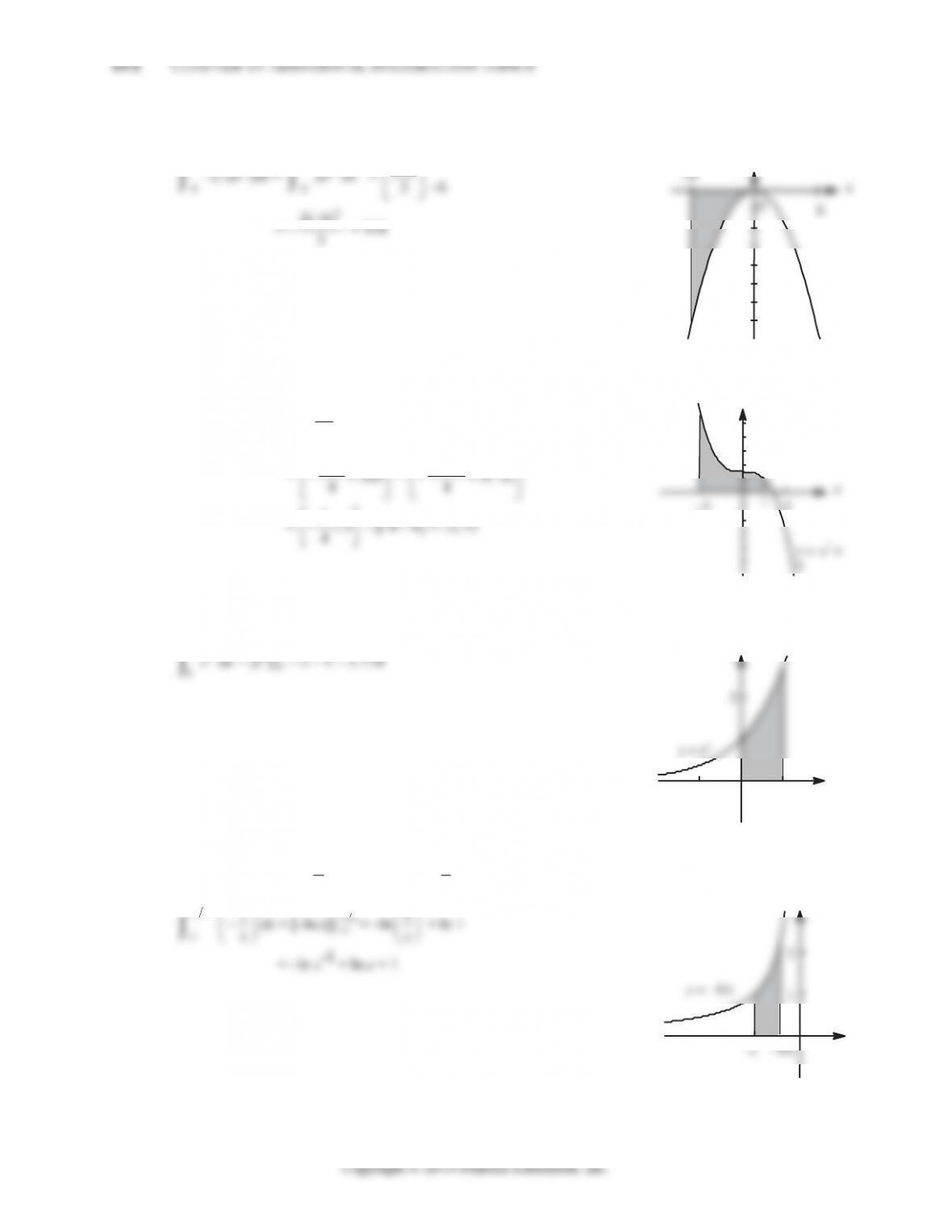
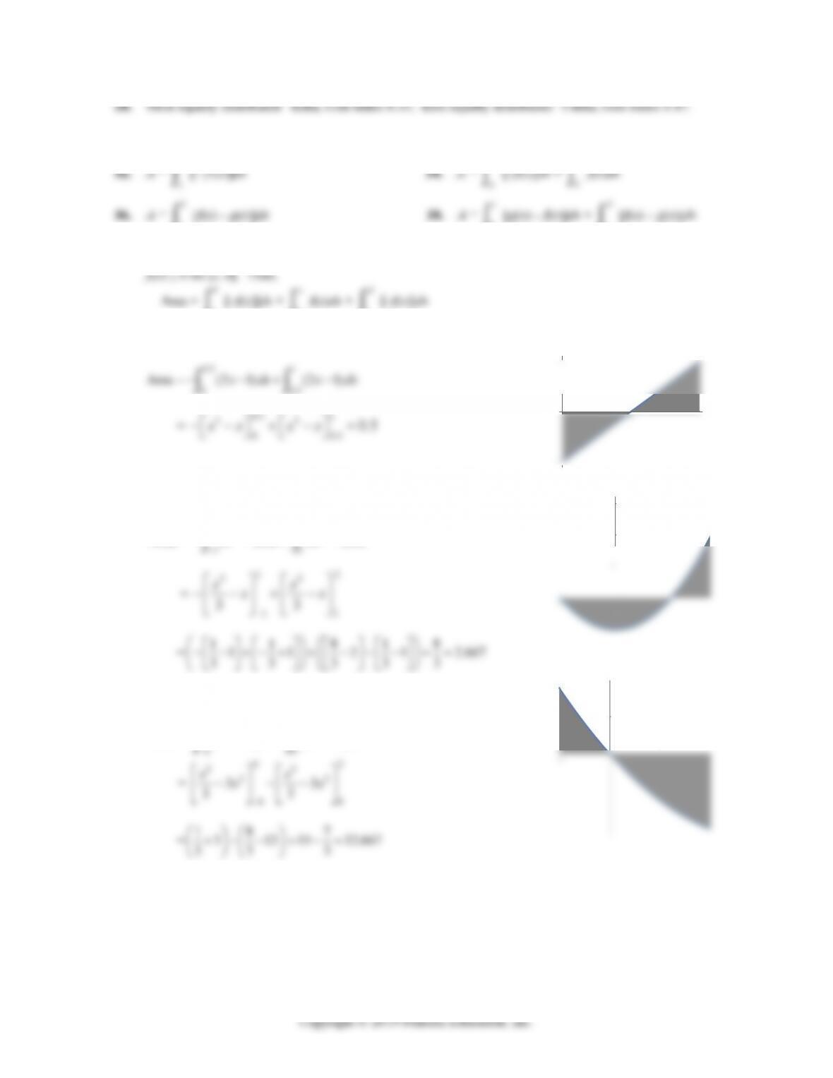
40. Find the x-intercepts b and c by solving f(x) = 0. Then observe that f(x) ≤ 0 on [a, b], f(x) ≥ 0 on [b, c], and
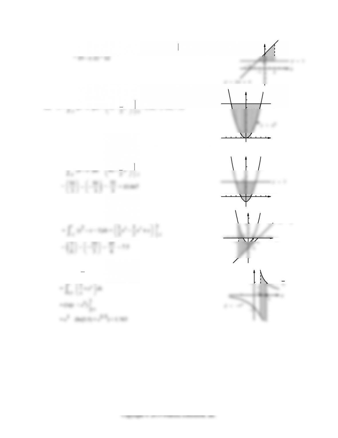
a
b
c
42. 21,0 1yx x
x
44. 21, 1 2yx x
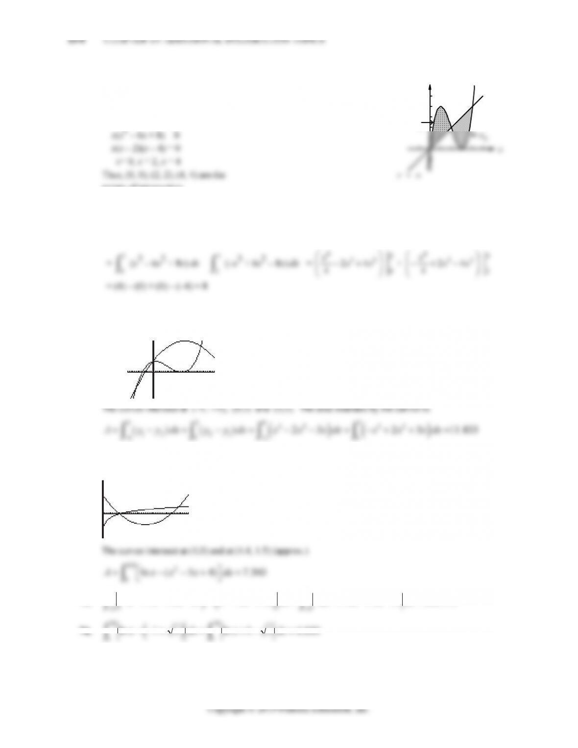
Area =
12
22
(1) (1)
x
dx x dx
=
12
33
11
33
xx
x
x
= 11 818
1 1 2 1 2.667
33 333
1
1
1 1
1
1
2
3
46. 26, 1 2yx x x
Area = 02
22
(6) (6)
x
xdx x xdx
4
13-4 CHAPTER 13: ADDITIONAL INTEGRATION TOPICS
48. A =
2
1
[(2x + 6) – 3]dx =
2
1
(2x + 3)dx = (x2 + 3x)2
1
6
-3
-1 2
y = 2x + 6
y
50. A =
3
[9 – x2]dx = 3
1
93
x
x
3
-3 3
y
x
9
0
52. A =
2
2
[3 – (x2 – 1)]dx
x
2
1
2
y
x
-2 -1 21
y = x2 – 1
54. A =
1
2
[(x2 – 1) – (x – 2)]dx
x
1
11
1
= 5
6
– 20
3
= 45
6 = 7.5
y
y = x – 2
-2
3
56. A =
1
0.5
1()
x
e
x
dx
1
y
EXERCISE 13-1 13-7
76. Solve
1
0
20.45
c
xxdx
for c.
1
21
1
2
c
cxx
78. Solve
1
0
20.37
c
xxdx
for c.
1
21
1
00
2
2210.37
21 1
c
cxx
xxdx cc
80.
15
5
R(t)dt =
15
5
2
100 4
25
t
t
dt = 100
15
5
225
t
tdt +
15
5
4 dt
Let u = t2 + 25, then du = 2t dt
t
2
t
1
82. To find the useful life, set R‘(t) = C‘(t) and solve for t:
5te-0.1t2 = 2t
e-0.1t2 =
2
5 = 0.4
13-8 CHAPTER 13: ADDITIONAL INTEGRATION TOPICS
3
0
[R‘(t) – C‘(t)]dt =
3
0
[5te-0.1t2 – 2t]dt = 5
3
0
te-0.1t2 dt – 2
3
0
t dt
Let u = –0.1t2, then du = –0.2t dt and
84. For 1962: f(x) = 3
10 x + 7
10 x2
Index of Income Concentration = 2
1
0
[x – f(x)]dx = 2
1
0
2
37
10 10
x
xx
dx = 2
1
0
2
77
10 10
x
x
dx
x
23
Index of Income Concentration = 2
1
0
[x – g(x)]dx = 2
1
0
2
11
22
x
xx
dx
x
1
1
x
86. For current Lorenz curve: f(x) = x2.3
Index of Income Concentration = 2
1
0
[x – f(x)]dx = 2
1
0
(x – x2.3)dx = 2
23.3
23.3
xx
1
0
11
x
13-10 CHAPTER 13: ADDITIONAL INTEGRATION TOPICS
16. (A) and (B) are equal:
10
0
2,000e0.05te0.12(10-t)dt = 2,000
10
0
e0.05te1.2e–0.12t dt = 2,000e1.2 10
0
e–0.07t dt
So, (A) and (B) are the same.
t
e
10
= 2,000
(C) 2,000e0.05 10
0
e0.12(10-t)dt = 2,000e0.05 10
0
e1.2e–0.12t dt = 2,000e0.05e1.2 10
0
e–0.12t dt
1
t
10
= 2,000
18. 20.
22. f(x) =
1
(1)
2if 0
otherwise
0
xx
3
1
3
(C)
13-12 CHAPTER 13: ADDITIONAL INTEGRATION TOPICS
44.
46. f(t) = 2,000e0.06t
0
0.06 e0.06t 35
0
3(e2.1 – 1) ≈ $238,872
48. f(t) = 2,000e0.06t, r = 0.0295, T = 6.
FV = e0.0295(6) 6
2,000e0.06te–0.0295t dt = 2,000e0.177 6
e0.0305t dt
6
0.0305 (e0.36 – e0.177) ≈ $15,717.92
50. Total Income =
6
0
2,000e0.06t dt = 2,000
0.06 (e0.06t)
6
0
= 100,000
3(e0.36 – 1) ≈ $14,444.31
52. Clothing store: f(t) = 12,000, r = 0.04, T = 10.
13-14 CHAPTER 13: ADDITIONAL INTEGRATION TOPICS
70. D(x) = 200 – 0.02x, p = 120
First, find
x
: 120 = 200 – 0.02
x
x
0
0
0
72.
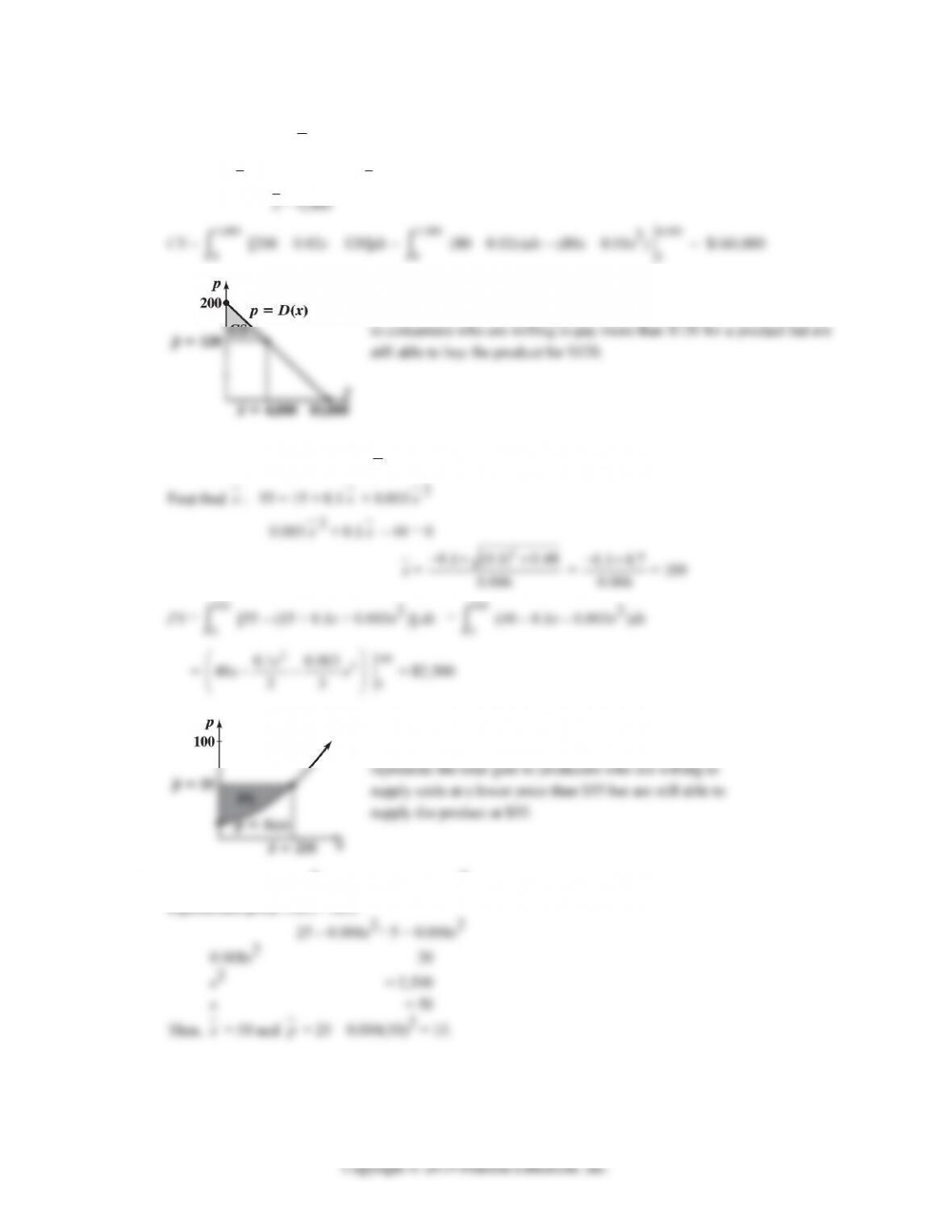
The shaded area is the consumers’ surplus and represents the total savings
74. p = S(x) = 15 + 0.1x + 0.003x2, p = 55.
x
x
x
x
x
x
x
0
76.
The area of the region PS is the producers’ surplus and
78. p = D(x) = 25 – 0.004x2; p = S(x) = 5 + 0.004x2
Equilibrium price: D(x) = S(x)
x
EXERCISE 13-2 13-15
CS =
50
0
[(25 – 0.004x2) – 15]dx =
50
0
(10 – 0.004x2)dx =
3
10 (0.004) 3
x
x
50
0
≈ $333
50
50
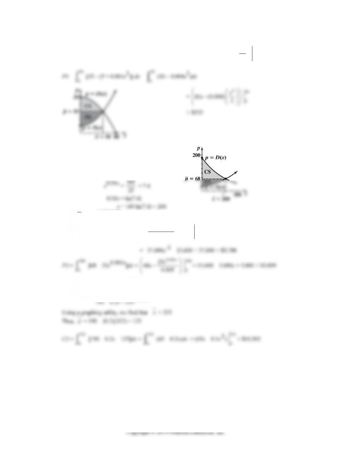
80. D(x) = 185e–0.005x and S(x) = 25e0.005x
Equilibrium price: D(x) = S(x)
185e–0.005x = 25e0.005x
Thus, p = 25e0.005(200) = 25e ≈ 68.
CS =
200
0
[185e–0.005x – 68]dx =
0.005
185 68
0.005
x
e
x
200
0
82. D(x) = 190 – 0.2x; S(x) = 25e0.005x
Equilibrium price: D(x) = S(x)
x
13-16 CHAPTER 13: ADDITIONAL INTEGRATION TOPICS
PS =
323
0
[125 – 25e0.005x]dx =
0.005
25
125 0.005
x
e
x
323
0
≈ $20,236
84. D(x) = 185e–0.005x; S(x) = 20 + 0.002x2
Equilibrium price: D(x) = S(x)
x
CS =
171.2
0
[185e–0.005x – 79]dx =
0.005
185 79
0.005
x
e
x
171.2
0
≈ $7,755
171.2
171.2
3
0.002
x
171.2
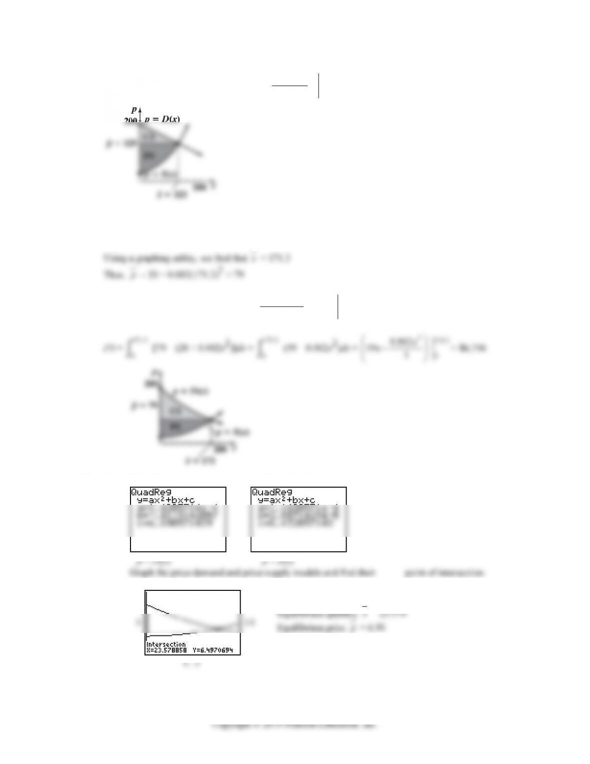
86. (A) Price–Demand Price–Supply
6.8
6.3
x
EXERCISE 13-3 13-17
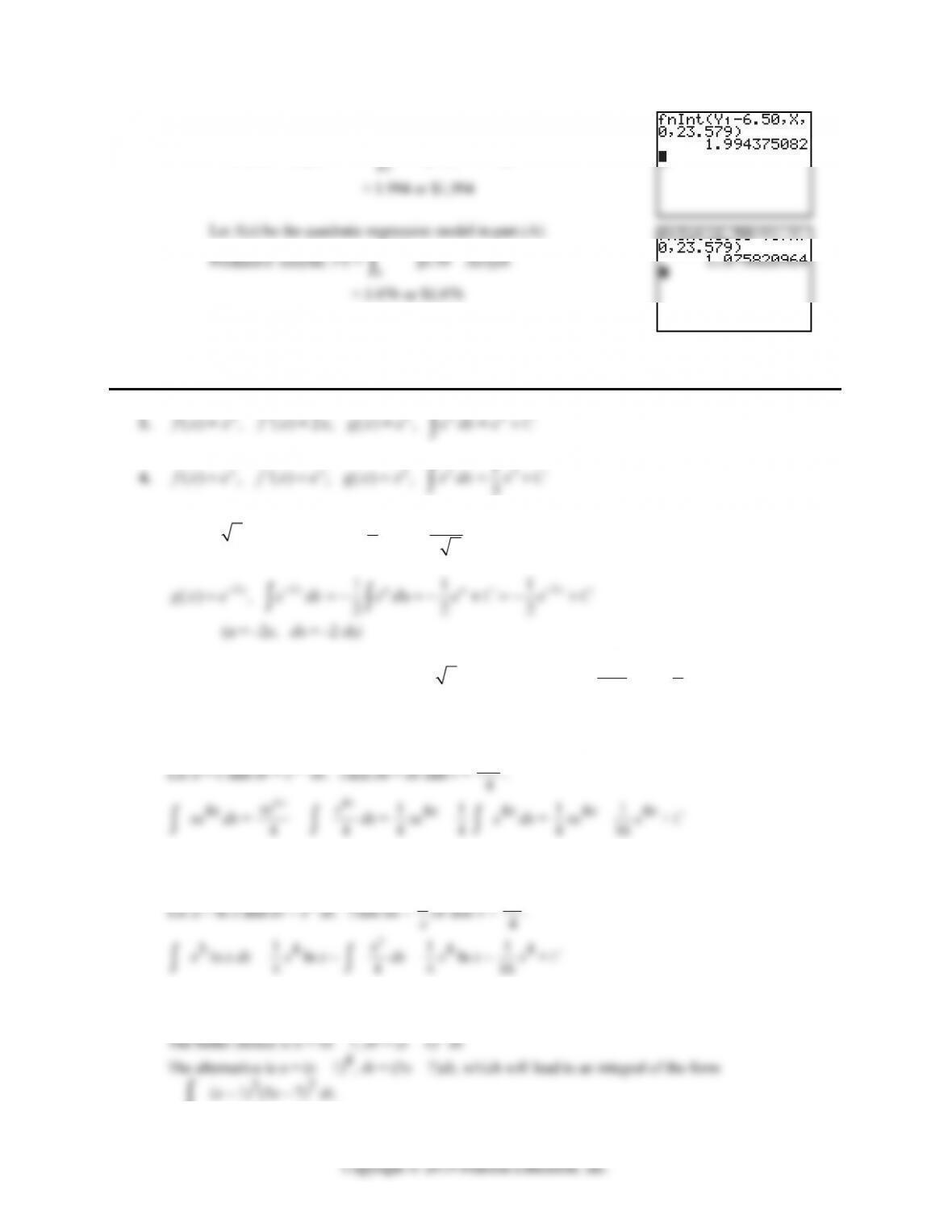
(B) Let D(x) be the quadratic regression model in part (A).
Consumers’ surplus: CS =
23.579
[D(x) – 6.50]dx
13-18 CHAPTER 13: ADDITIONAL INTEGRATION TOPICS
Let u = 5x – 7 and dv = (x – 1)4 dx. Then du = 5 dx and
16.
(x – 1)e-x dx
18.
xe-x2dx
20.
1
0
(x + 1)ex dx
22.
2
1
ln 2
x
dx
Let u = ln 2
x
and dv = dx. Then du =
2
1
x
· 1
2dx = 1
x
dx and v = x.
x
x
x
x
x
24.
2
35
x
xdx =
(x3 + 5)-1x2 dx
Let u = x3 + 5, then du = 3x2 dx.
x
13-20 CHAPTER 13: ADDITIONAL INTEGRATION TOPICS
23 3 3 3
111
(3 2)( 1) ( 1) (3 2) ( 1) (3) ( 1) (3 2) ( 1)
333
x
xdxx x x dxx x xdx
x
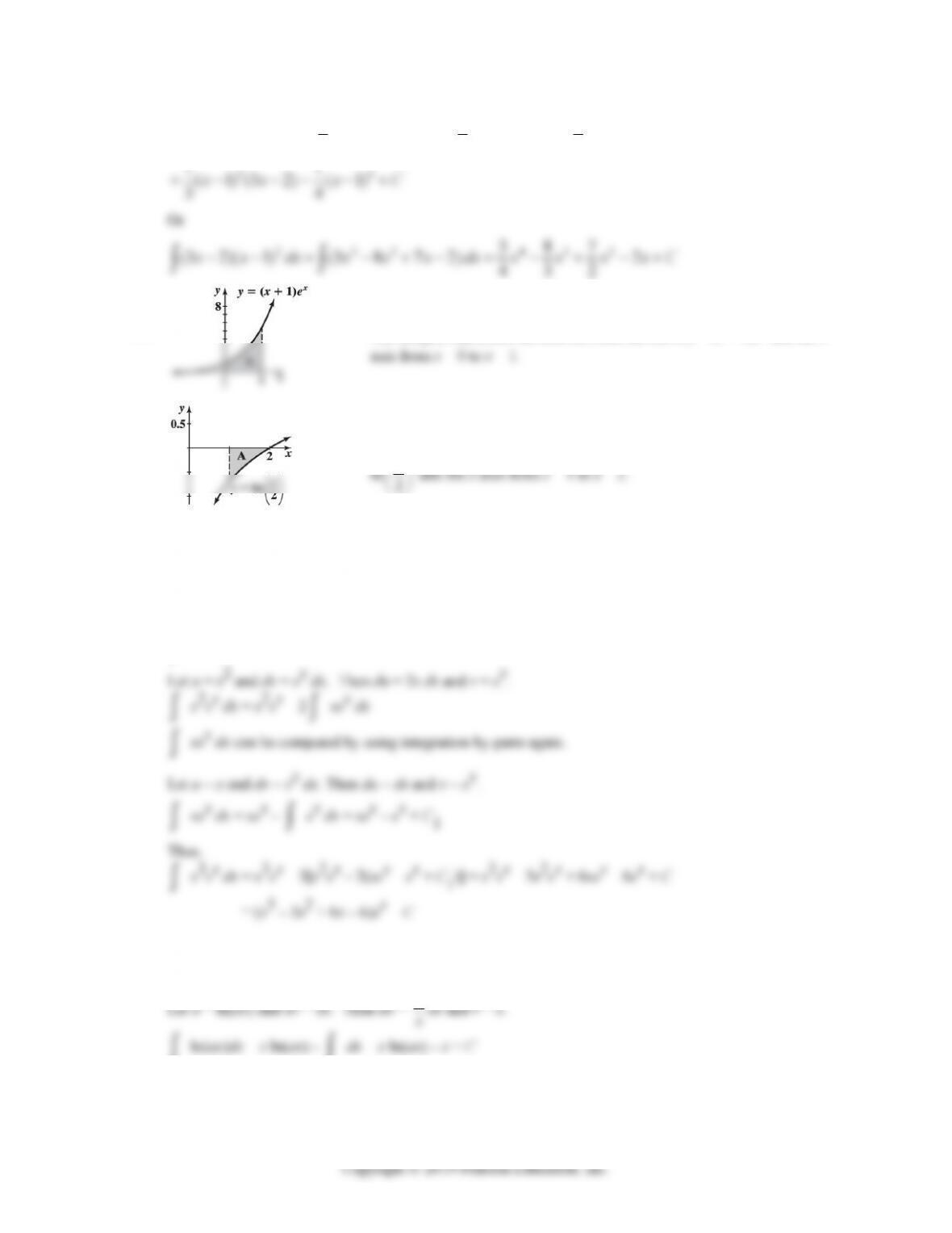
36.
The integral represents the area between the curve y = (x + 1)ex and the x
38.
The integral represents the negative of the area between the curve y =
x
40.
x3ex dx
Let u = x3 and dv = ex dx. Then du = 3x2 dx and v = ex.
x3ex dx = x3ex –
3x2ex dx = x3ex – 3
x2ex dx
x2ex dx can be computed by using integration-by-parts again.
42.
ln(ax)dx, a > 0
x