CHAPTER 13
Waiting Lines and Queuing Theory Models
TEACHING SUGGESTIONS
Teaching Suggestion 13.1: Topic of Queuing.
Here is a chapter that all students can relate to. Ask about student experiences in lines. Stress that
Teaching Suggestion 13.2: Cost of Waiting Time from an Organizational Perspective.
Students should realize that different organizations place different values on customer waiting
Teaching Suggestion 13.3: Use of Poisson and Exponential Probability Distributions to
Describe Arrival and Service Rates.
These two distributions are very common in basic models, but students should not take their
as exponential, normal, or Erlang) are often more valid.
Teaching Suggestion 13.4: Balking and Reneging Assumptions.
Note that most queuing models assume that balking and reneging are not permitted. Since we
Teaching Suggestion 13.5: Use of Queuing Software.
The Excel QM and QM for Windows queuing software modules are among the easiest models in
Teaching Suggestion 13.6: Importance of Lq and Wq in Economic Analysis.
Although many parameters are computed for a queuing study, the two most important ones are
Lq and Wq when it comes to an actual cost analysis.
Teaching Suggestion 13.7: Teaching the New England Foundry Case.
ALTERNATIVE EXAMPLES
Alternative Example 13.1: A new shopping mall is considering setting up an information desk
manned by one employee. Based on information obtained from similar information desks, it is
believed that people will arrive at the desk at the rate of 20 per hour. It takes an average of 2
minutes to answer a question. It is assumed that arrivals are Poisson and answer times are
exponentially distributed.
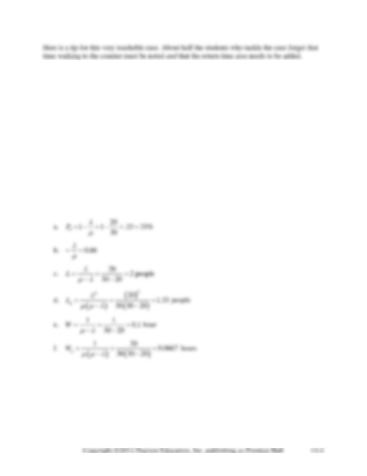
a. Find the probability that the employee is idle.
b. Find the proportion of the time that the employee is busy.
c. Find the average number of people receiving and waiting to receive information.
d. Find the average number of people waiting in line to get information.
e. Find the average time a person seeking information spends at the desk.
f. Find the expected time a person spends just waiting in line to have a question answered.
ANSWER: = 20/hour
= 30/hour
Alternative Example 13.2: In Alternative Example 13.1, the information desk employee earns
a. The average person waits 0.0667 hour and there are 160 arrivals per day. So total waiting
time = (160)(0.0667) = 10.67 hours @ $12/hour, implying a waiting cost of $128/day.
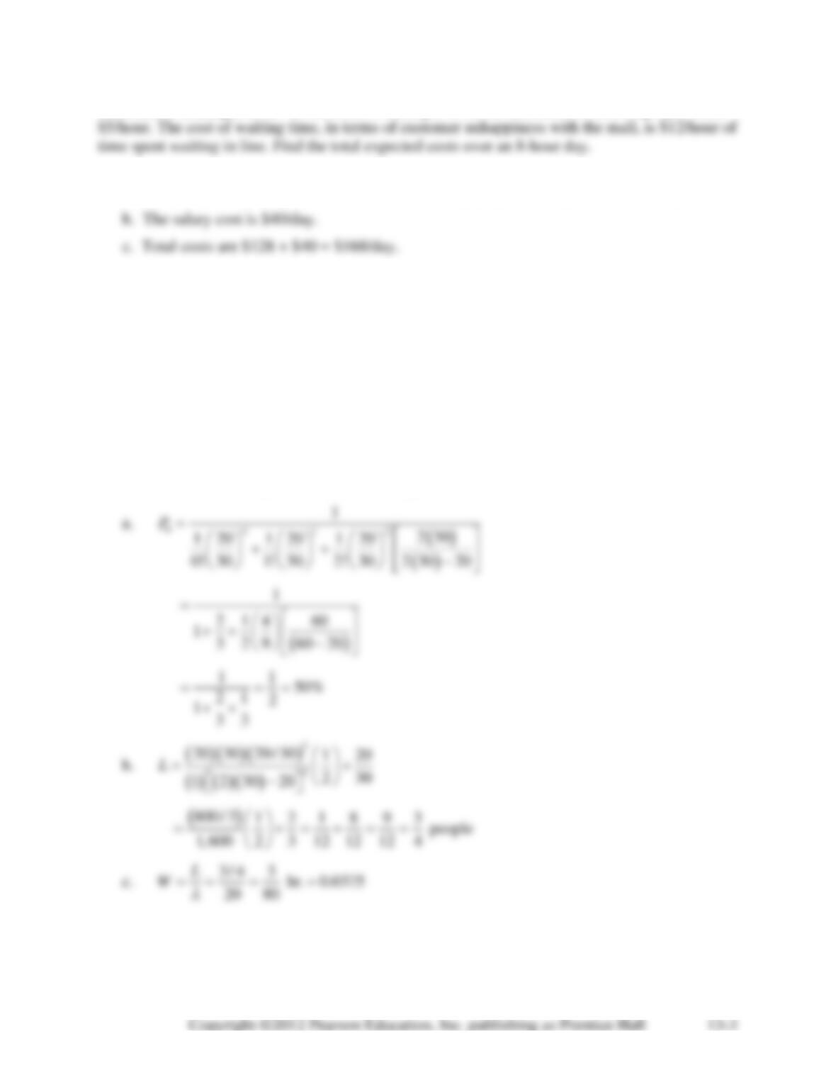
Alternative Example 13.3: A new shopping mall is considering setting up an information desk
manned by two employees. Based on information obtained from similar information desks, it is
believed that people will arrive at the desk at the rate of 20 per hour. It takes an average of 2
minutes to answer a question. It is assumed that arrivals are Poisson and answer times are
exponentially distributed.
a. Find the proportion of the time that the employees are idle.
b. Find the average number of people waiting in the system.
c. Find the expected time a person spends waiting in the system.
ANSWER: = 20/hour,
= 30/hour, M = 2 open channels (servers).
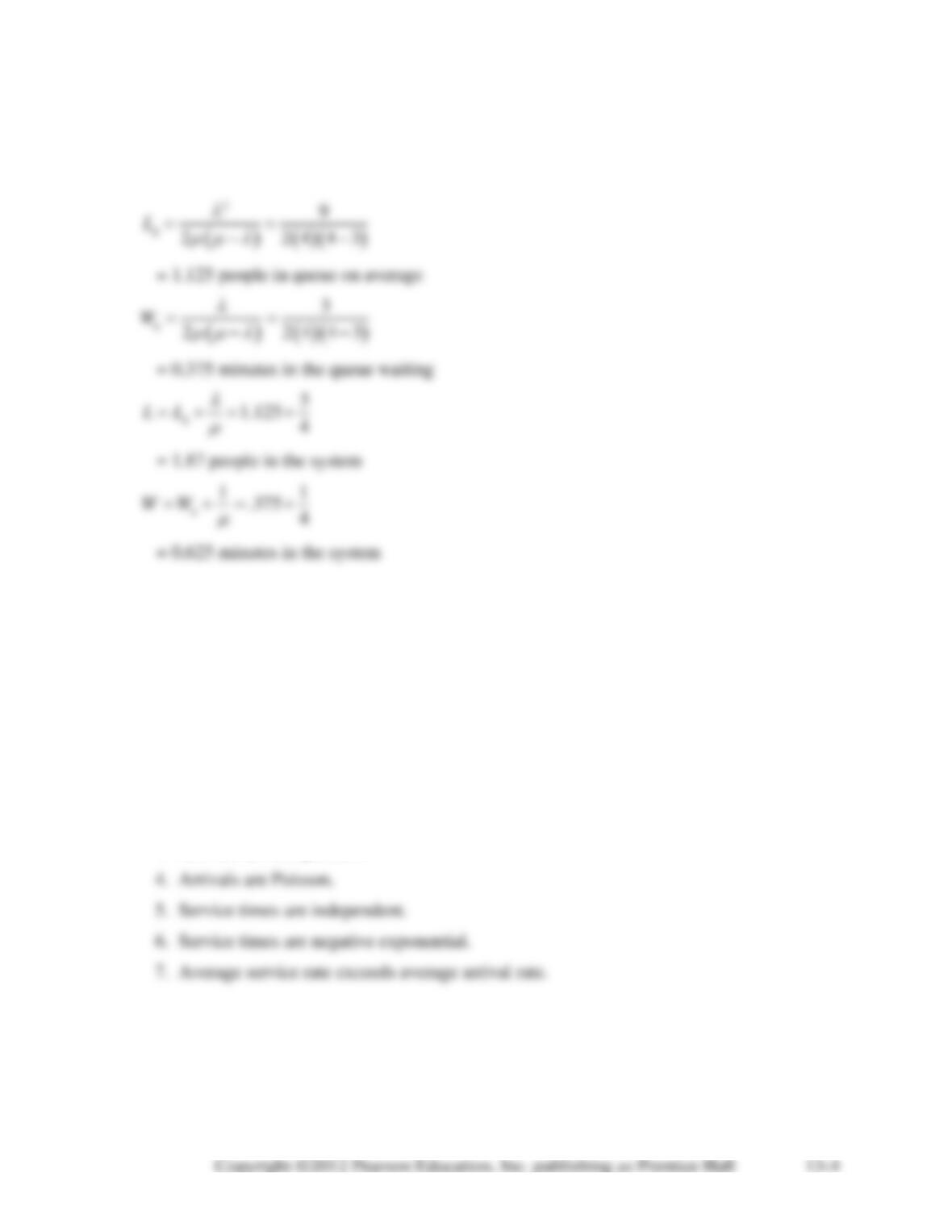
Alternative Example 13.4: Three students arrive per minute at a coffee machine that dispenses
exactly 4 cups/minute at a constant rate. Describe the operating system parameters.
ANSWER: = 3/minute
= 4/minute
SOLUTIONS TO DISCUSSION QUESTIONS AND PROBLEMS
13-1. The waiting line problem concerns the question of finding the ideal level of service that an
organization should provide. The three components of a queuing system are arrivals, waiting
line, and service facility.
13-2. The seven underlying assumptions are:
1. Arrivals are FIFO.
2. There is no balking or reneging.
3. Arrivals are independent.
13-3. The seven operating characteristics are:
1. Average number of customers in the system (L)
2. Average time spent in the system (W)
13-4. If the service rate is not greater than the arrival rate, an infinite queue will eventually build
up.
13-5. First-in, first-out (FIFO) is often not applicable. Some examples are (1) hospital
emergency rooms, (2) an elevator, (3) an airplane trip, (4) a small store where the shopkeeper
13-6. Examples of finite queuing situations include (1) a firm that has only 3 or 4 machines that
13-7. a. Barbershop: usually a single-channel, multiple-service system (if there is more than one
barber).
Arrivals = customers wanting haircuts
b. Car wash: usually either a single-channel, single-server system, or else a system with
each service bay having its own queue.
Arrivals = dirty cars or trucks
c. Laundromat: basically a single-channel, multiserver, two-phase system.
d. Small grocery store: usually a single-channel, single-server system.
Arrivals = customers buying food items
13-8. The waiting time cost should be based on time in the queue in situations where the
customer does not mind how long it takes to complete service once the service starts. The classic
example of this is waiting in line for an amusement park ride.
13-9. The use of Poisson to describe arrivals:
a. Cafeteria: probably not. Most people arrive in groups and eat at the same time.
b. Barbershop: probably acceptable, especially on a weekend, in which case people arrive at
the same rate all day long.
c. Hardware store: okay.
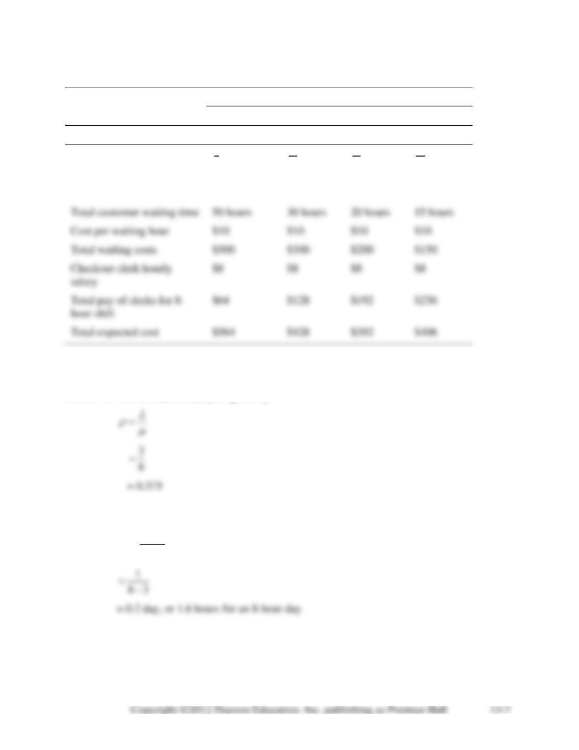
13-10
NUMBER OF CHECKOUT CLERKS
1
2
3
4
Number of customers
300
300
300
300
Average waiting time
1
6
hour
1
10
hour
1
15
hour
1
20
hour
per customer
(10 minutes)
(6
minutes)
(4
minutes)
(3
minutes)
$500
$300
$200
$150
Checkout clerk hourly
salary
Total pay of clerks for 8-
$564
$428
$392
$406
Optimal number of
checkout clerks on duty = 3
13-11. a. The utilization rate,
, is given by
b. The average down time, W, is the time the machine waits to be serviced plus the time
taken to perform the service.
1
W
=−
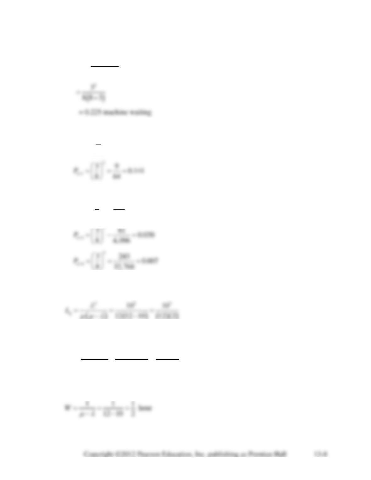
c. The number of machines waiting to be served, Lq, is, on average,
( )
2
q
L
=−
d. Probability that more than one machine is in the system
1k
nk
P
+
=
Probability that more than two machines are in the system:
3
2
3 27 0.053
8 512
n
P
= = =
13-12.
= 10 cars/hour,
= 12 cars/hour.
a. The average number of cars in line, Lq, is given by
= 4.167 cars
b. The average time a car waits before it is washed, Wq, is given by
( ) ( ) ( )( )
10 10
12 12 10 12 2
q
W
= − =
−−
= 0.4167 hour
c. The average time a car spends in the service system, W, is given by
d. The utilization rate,
, is given by
10 0.8333
12
= = =
e. The probability that no cars are in the system, P0, is given by:
13-13.
= 210 patrons/hour,
= 280 patrons/hour.
a. The average number of patrons waiting in line, Lq, is given by
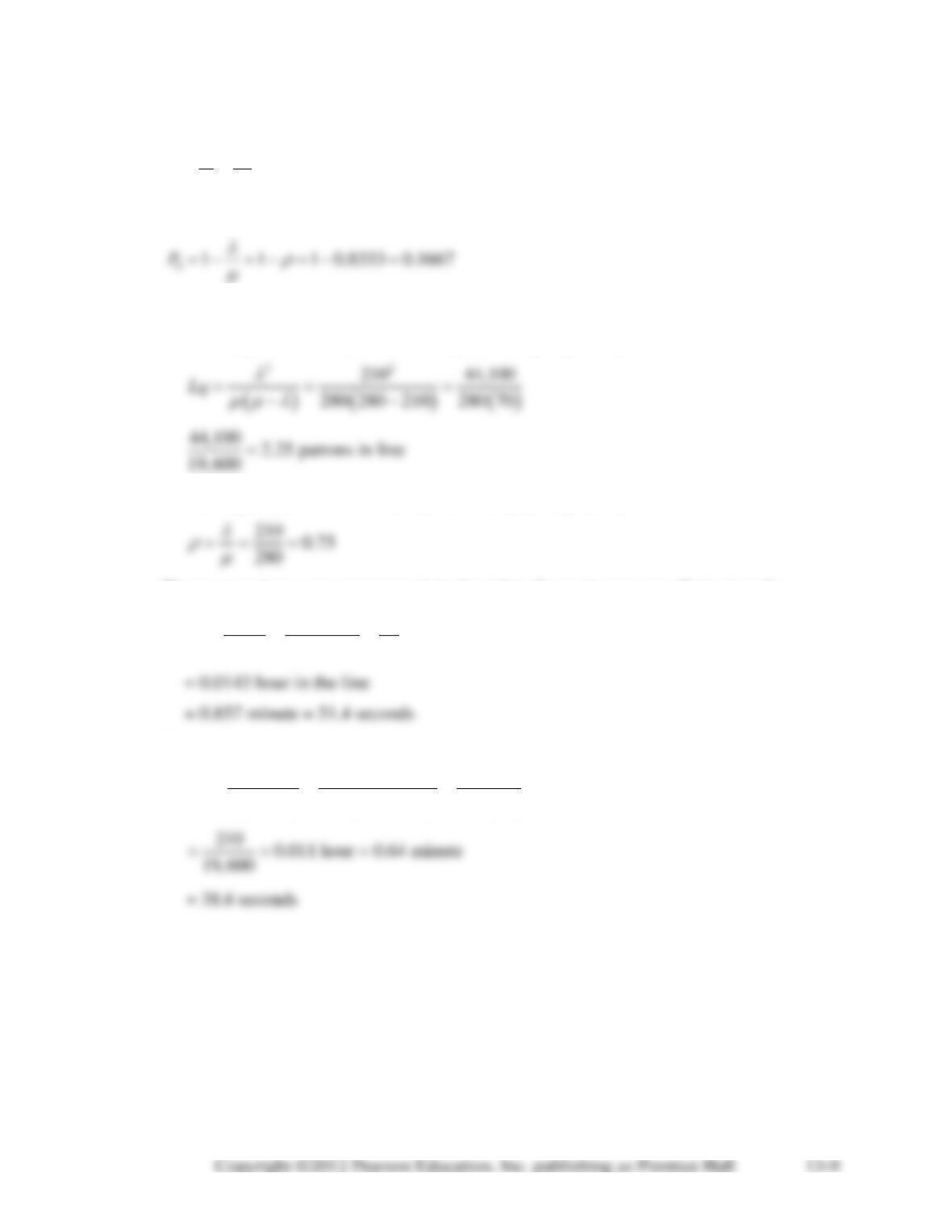
b. The average fraction of time the cashier is busy,
, is given by
c. The average time a customer spends in the ticket-dispensing system, W, is given by
1 1 1
280 210 70
W
= = =
−−
d. The average time spent by a patron waiting to get a ticket, Wq, is given by
( ) ( ) ( )
210 210
280 280 210 280 70
q
W
= = =
−−
e. The probability that there are more than two people in the system, Pn>2, is given by
1k
nk
P
+
=
The probability that there are more than three people in the system, Pn > 3, is given by
13-14.
= 4 students/minute,
=
60
12
= 5 students/minute
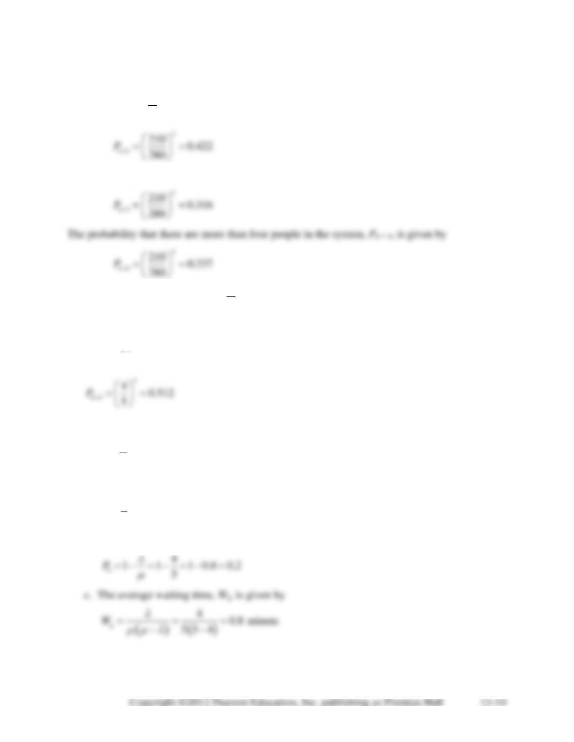
a. The probability of more than two students in the system, Pn > 2, is given by
1k
nk
P
+
=
The probability of more than three students in the system, Pn>3, is given by
4
3
40.410
5
n
P
==
The probability of more than four students in the system, Pn>4, is given by
5
4
40.328
5
n
P
==
b. The probability that the system is empty, P0, is given by
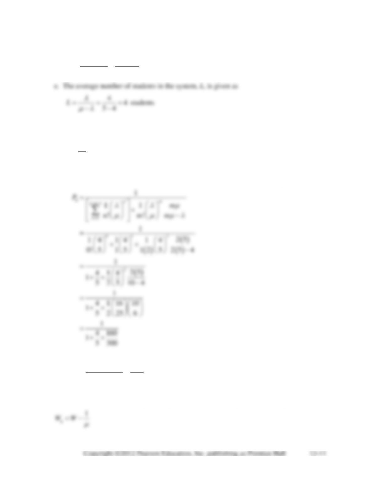
d. The expected number of students in the queue, Lq, is given by
( ) ( )
2
43.2
5 5 4
q
L
= = =
−−
students
f. Adding a second channel, we have
= 4 students/minute
60 5
12
==
students/minute
m = 2
f (part b). The probability that the two-channel system is empty, P0, is given by
or
0
11
0.429
1 0.8 0.53 2.33
P= = =
++
Thus the probability of an empty system when using the second channel is 0.429.
f (part c). The average waiting time, Wq, for the two-channel system is given by
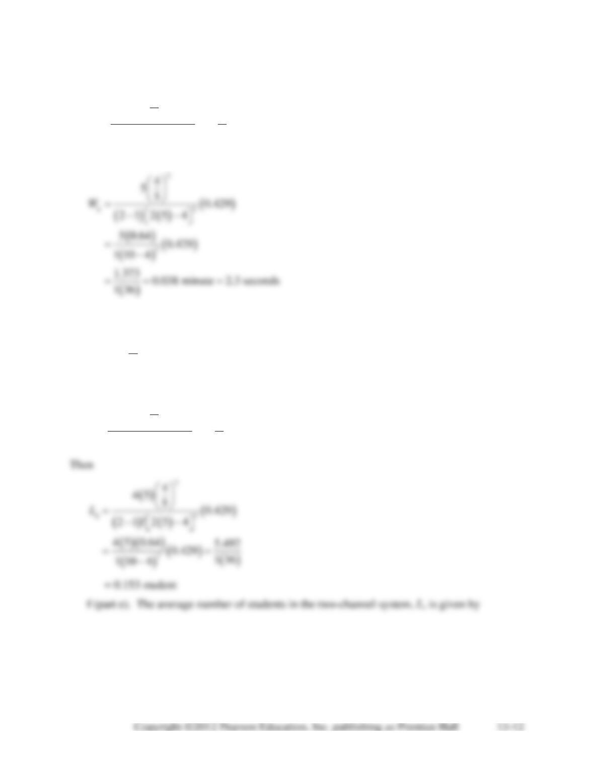
where
( ) ( )
0
2
1
1!
m
WP
mm
=+
−−
Then
f (part d). The average number of students in the queue for the two-channel system, Lq, is
given by
q
LL
=−
where
( ) ( )
0
2
1!
m
LP
mm
=+
−−
13-15.
= 30 trucks/hour,
= 35 trucks/hour.
a. The average number of trucks in the system, L, is given by
30 30 6 trucks in the system
35 30 5
L
=−
= = =
−
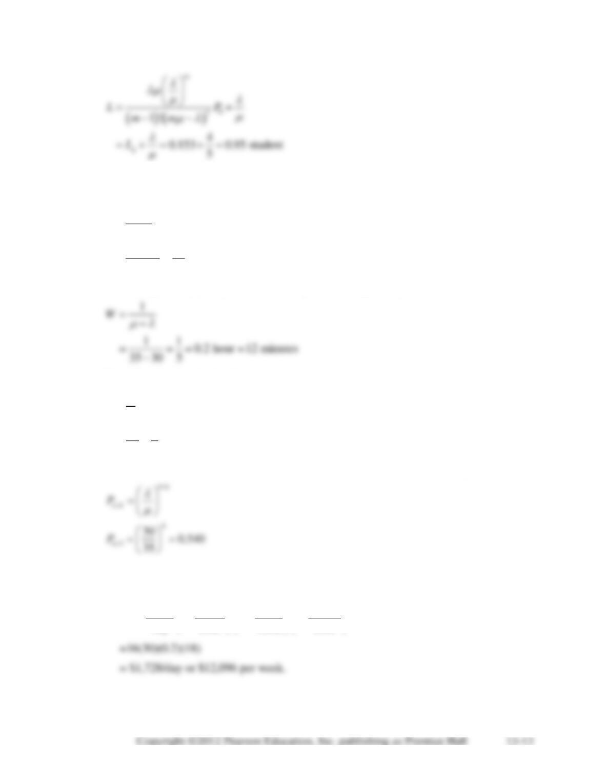
b. The average time spent by a truck in the system, W, is given by
c. The utilization rate for the bin area,
, is given by
30 6 0.857
35 7
=
= = =
d. The probability that there are more than three trucks in the system, Pn > 3, is given by
Thus the probability that there are more than three (four or more) trucks in the system is 0.540.
e. Unloading cost:
hours trucks hours dollars
16 30 0.2 18
day hour truck hour
M
C
=
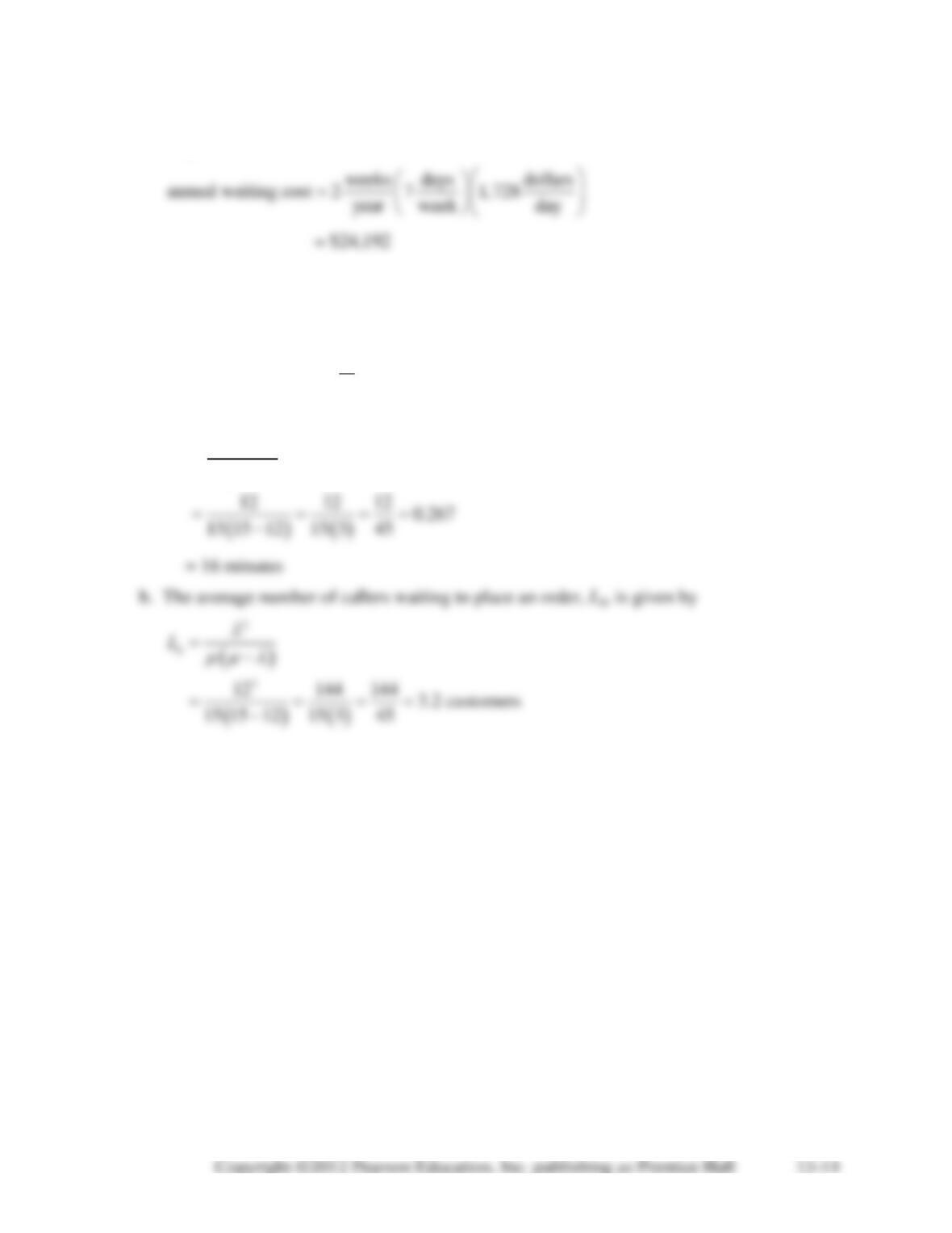
f. Enlarging the bin will cut waiting costs by 50% next year. First, we must compute annual
waiting costs:
Note this weekly cost is what was found in part e of this problem. Enlarging the bin will cut
waiting costs by 50% next year, resulting in a savings of $12,096. Since the cost of enlarging the
bin is only $9,000, the cooperative should proceed to enlarge the bin. The net savings is $3,096
($12,096 – $9,000).
13-16.
= 12 calls/hour,
=
60
4
= 15 calls/hour.
a. The average time the catalog customer must wait, Wq, is given by
( )
q
W
=−