College Mathematics: Learning Worksheets Chapter 13
Name ________________________________ Date ______________ Class ____________
Goal: To find the area between two curves
In Problems 1–7, find the area bounded by the graphs of the indicated equations over the
given interval (when stated). Compute answers to three decimals, if necessary.
1. 3
82;yx=− 0;y06x≤≤
3
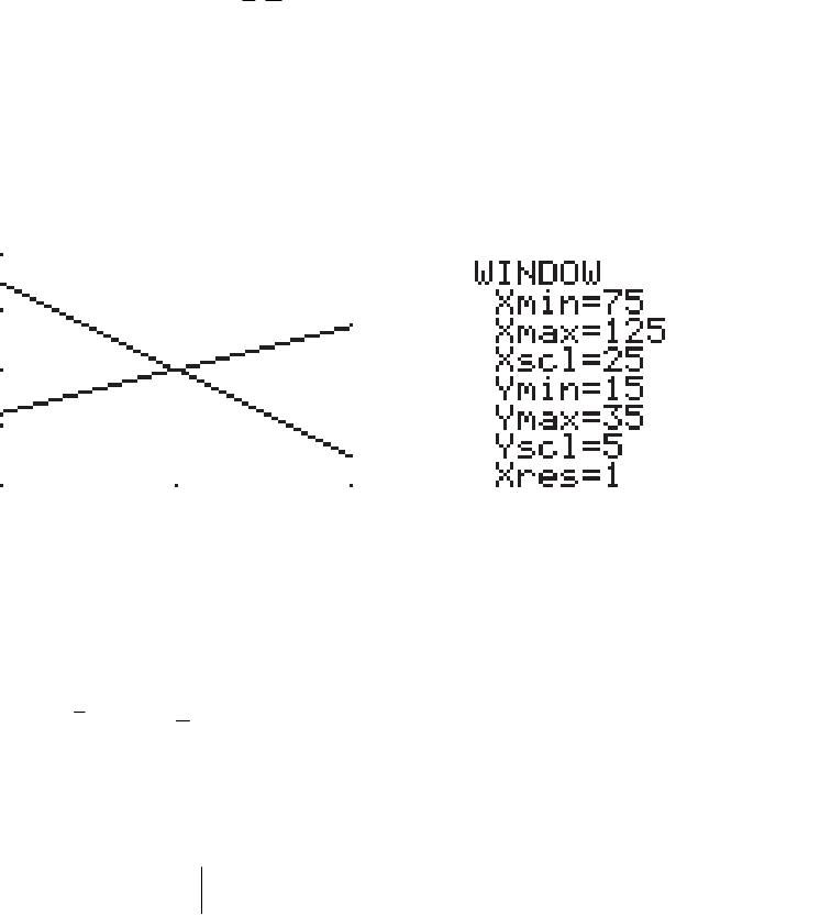
3
3
31
4
2
2
820
82
x
x
x
x
32
232
2
32
232
2
32
6
33
0
6
33
0
[0 (8 2)] [8 2 0]
[ 8 2] [8 2]
Axdxxdx
Axdxxdx
=−−+ −−
∫∫
=−+ + −
∫∫
Section 13-1 Area Between Curves
Theorem: Area Between Two Curves
If f and g are continuous and () ()
f
xgxover the interval [a, b], then the area
bounded by ()yfxand ()ygxfor axbis given exactly by
[() ()] .
b
a
Afxgxdx
Definition: Gini Index of Income Concentration
2. 3
29;yx 0;y32x
3
3
39
2
9
32
290
29
x
x
x
x
9
32
9
32
9
32
9
32
2
33
3
2
33
3
[2 90] [0(2 9)]
[ 2 9] [2 9]
Axdx xdx
Axdxxdx
34
29
32
() (3)
(2)
9(2) 9( )
3. 85;
x
ye=− 0;y02x
2
0
[8 5 0]
x
Ae dx
=−−
∫

377
4. 37;yx 4;y 70x
11
3
43 7
11 3
x
x
x
11
311
3
11
311
3
11
0
7
0
7
0
[( 4) (3 7)] [3 7 ( 4)]
[3 11] [3 11]
Axdxxdx
Axdxxdx
2
11 2
311
3
3( ) 3( 7)
2
5. 210;yx=− 15y=
The first step in the problem is to find where the two functions intersect. Set both
equations equal to each other to find the intersection points.
2
10 15
x
−=
A graph of 210yx=−and 15y=shows that 2
15 10x≥−on the interval [–5, 5].
Now find the area using the definite integral from –5 to 5.
College Mathematics: Learning Worksheets Chapter 13
33
(5) ( 5)
25(5) 25( 5)
33
A
⎛⎞⎛ ⎞
−
=− + −− + −
⎜⎟⎜ ⎟
⎜⎟⎜ ⎟
6. 22;yx 5;yx 32x
22
3
22
3
[( 2) ( 5)]
[3]
Ax xdx
Axxdx
7. 57;yx=+ 52;yx=− 53x
3
5
[(57)(52)]
Ax xdx
−
=+−−
∫
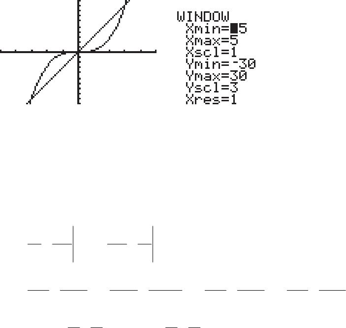
8. 3;
y
x9yx
Based on the graph above, the points of intersection are –3, 0, and 3, therefore, the
area between the curves is
03
33
30
03
33
30
[( ) (9 )] [(9 ) ( )]
[9] [9 ]
Axxdxxxdx
Axxdxxxdx
380
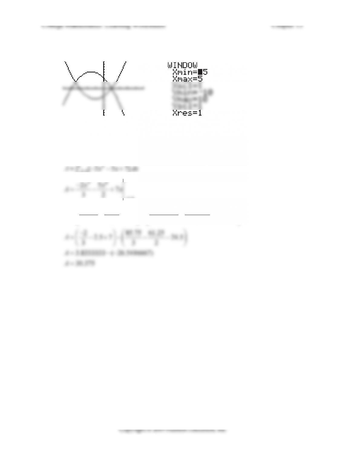
9. 223;yx x 234;yx x
Based on the graph above, the points of intersection are –3.5 and 1, therefore, the area
between the curves is
122
3.5
3.5
1
3.5
[( 3 4) ( 2 3)]
Axxxxdx
32 3 2
2(1) 5(1) 2( 3.5) 5( 3.5)
7(1) 7( 3.5)
32 3 2
A

College Mathematics: Learning Worksheets Chapter 13
Name ________________________________ Date ______________ Class ____________
Goal: To solve application problems that involve business and economics
Section 13-2 Applications in Business
and Economics
Definitions:
1. Total Income for a Continuous Income Stream
f
a
f
2. Future Value of a Continuous Income Stream
If ( )
f
tis the rate of flow of a continuous stream, 0 ,tT and if the income
3. Consumers’ Surplus
p
4. Producers’ Surplus
If
(, )
x
pis a point on the graph of the price–supply equation ( ),
p
Sxthen
p

College Mathematics: Learning Worksheets Chapter 13
In Problems 1–3, evaluate each definite integral to two decimals.
1. 67
0
t
edt
−
∫
6
0.14
=
2. 70.03(3 2 )
0
t
edt
77
0.03(3 2) 0.03(3) 0.06
00
7
0.09 0.06
1
0.06
t
t
edteedt
ee
3. 50 0.05 0.07(50 )
0600 tt
ee dt
−
∫
50 50
0.05 0.07(50 ) 0.05 3.5 0.07
00
50 3.5 0.02
50
3.5 0.02
600 600
600
tt tt
t
t
ee dt ee dt
eedt
−−
−
−
=
∫∫
=∫
3.5 0.02
50 0.05 0.07
(5
3.5
0
)1
600 0.02
600 ( 18.
60
39397 50)
0
tt t
eee
t
ed
e
−−
⎜⎟
=−
≈
−+

383
4. Find the total income produced by a continuous income stream in the first 6 years if
the rate of flow if 0.07
( ) 500 .
t
ft e=
60.07
Total income ( )
500
0.07
b
a
t
ftdt
edt
e
ee
=∫
=∫
=
=−
5. Find the future value, at 3.5% interest, compounded continuously for 5 years, of the
continuous income stream with rate of flow 0.05
( ) 3000 .
t
ft e
0
5
(0.035)(5) 0.05 0.035
5
0.175 0.015
0.175 5
0
0.175 0.015(5) 0.015(0)
()
0.015
T
rT rt
tt
t
FV e f t e dt
−
−
=∫
⎝⎠
6. Find the consumers’ surplus at a price level of $160pfor the price–demand
equation ( ) 460 0.06 .
p
Dx x
First, find
x
by substituting the value $160pinto the price–demand equation.
460 0.06
p
x

College Mathematics: Learning Worksheets Chapter 13
384
Now use the consumers’ surplus definition.
0
[() ]
x
CS D x p dx
7. Find the producers’ surplus at a price level of $98pfor the price–supply equation
2
( ) 10 0.1 0.0003 .
p
Sx x x
First, find
x
by substituting the value $98pinto the supply–demand equation.
p
x
Using the quadratic formula will yield that 400.x
Now use the producers’ surplus definition.
0
400 2
0
[()]
[98 (10 0.1 0.0003 )]
x
PS p S x dx
PS x x dx
385
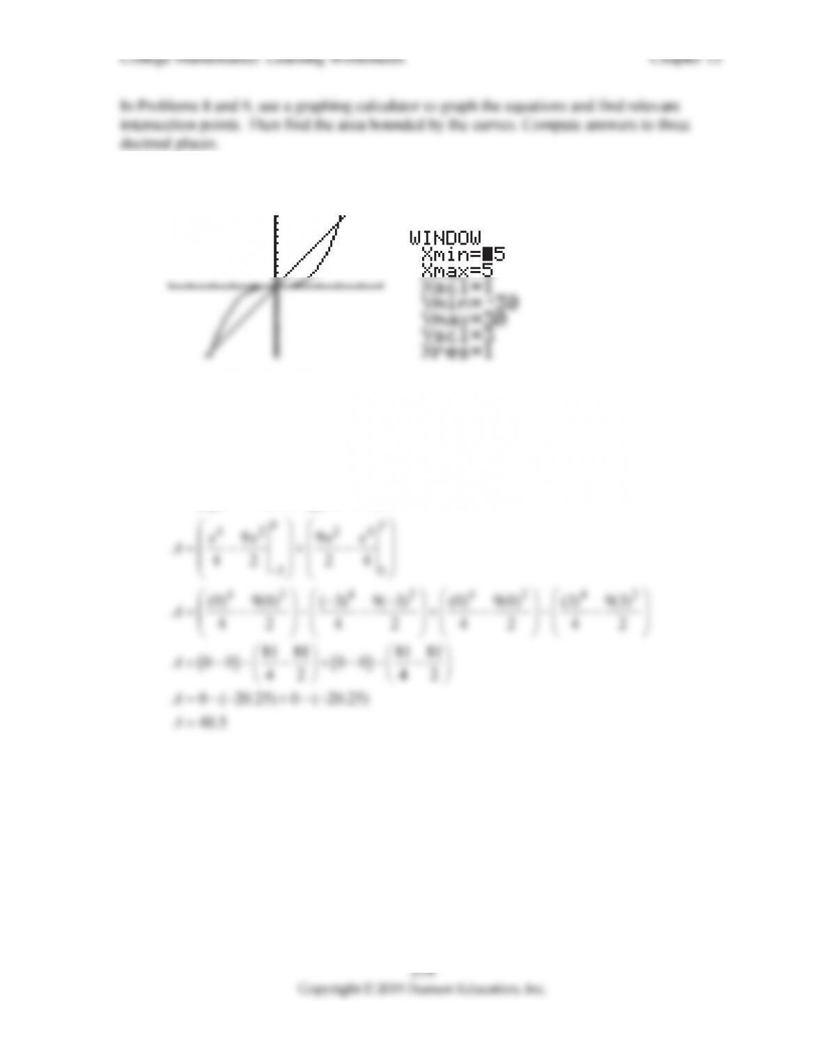
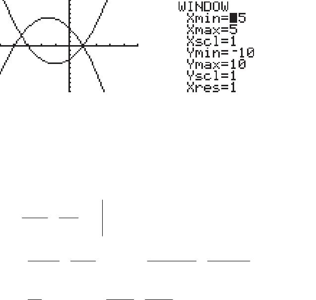
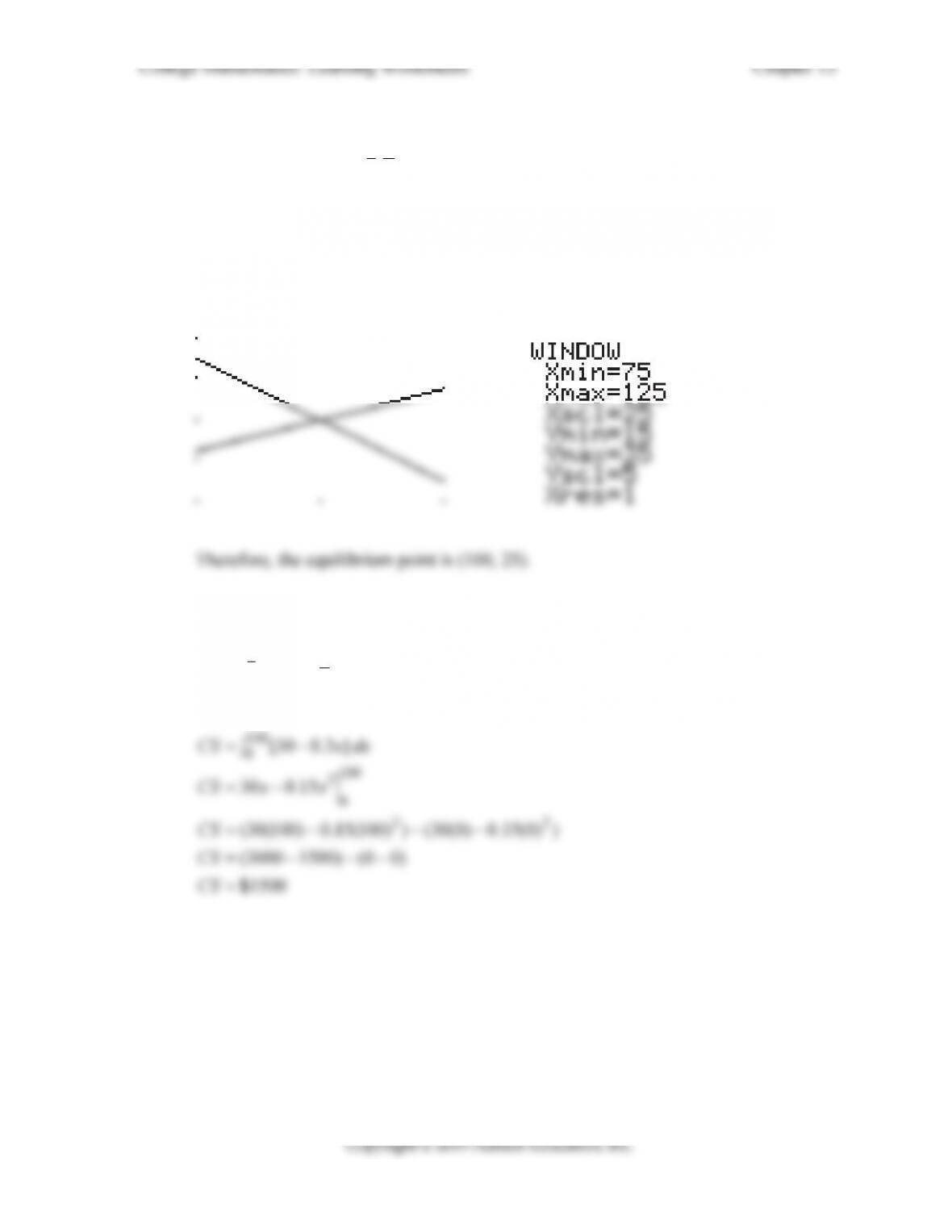
8. Find the consumers’ surplus and the producers’ surplus at the equilibrium price level
for the given price–demand and price–supply equations. Include a graph that shows
the equilibrium point (, ).
x
p Round all values to the nearest integer if necessary.
( ) 55 0.3
p
Dx x ( ) 10 0.15
p
Sx x
The equilibrium point is also the point of intersection. Through a process that
narrows the window required to see the point of intersection, the graph will look as
follows
The consumers’ surplus will be
0
100
0
[() ]
[55 0.3 25]
x
CS D x p dx
CS x dx