Chapter 17
17 – 12
Model Title: MARKOWITZ
Variable Value Reduced Cost
R1 18.95698 0.000000
RBAR 10.00000 0.000000
R2 11.51205 0.000000
R3 5.643902 0.000000
R4 9.728075 0.000000
19.
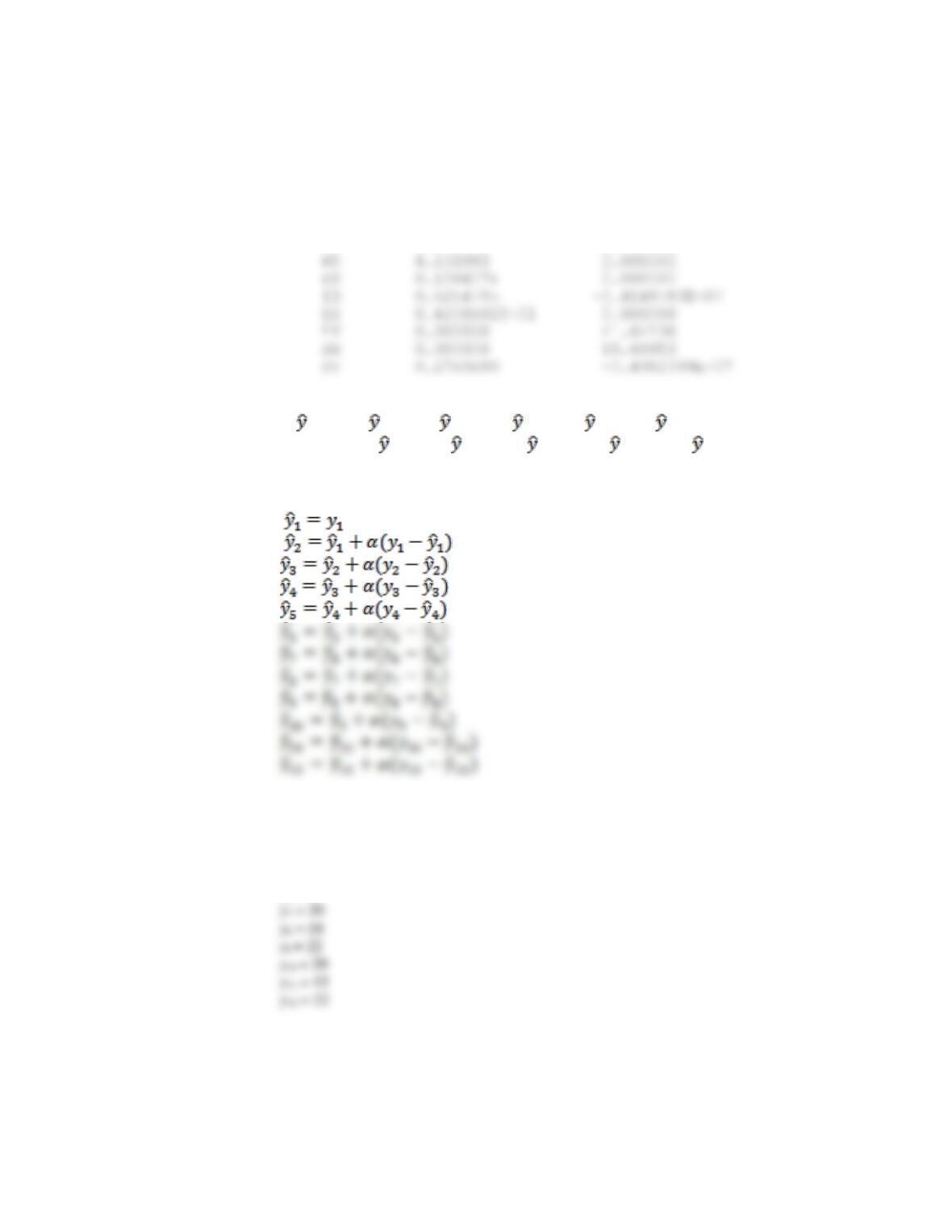
Min = (y2 – 2)2 + (y3 – 3)2 + (y4 – 4)2 + (y5 – 5)2 + (y6 – 6)2 + (y7 – 7)2
+ (y8 – 8)2 + (y9 – 9)2 + (y10 – 10)2 + (y11 – 11)2 + (y12 – 12)2
s.t.
y1 = 17
y2 = 21
y3 = 19
y4 = 23
y5 = 18
y6 = 16
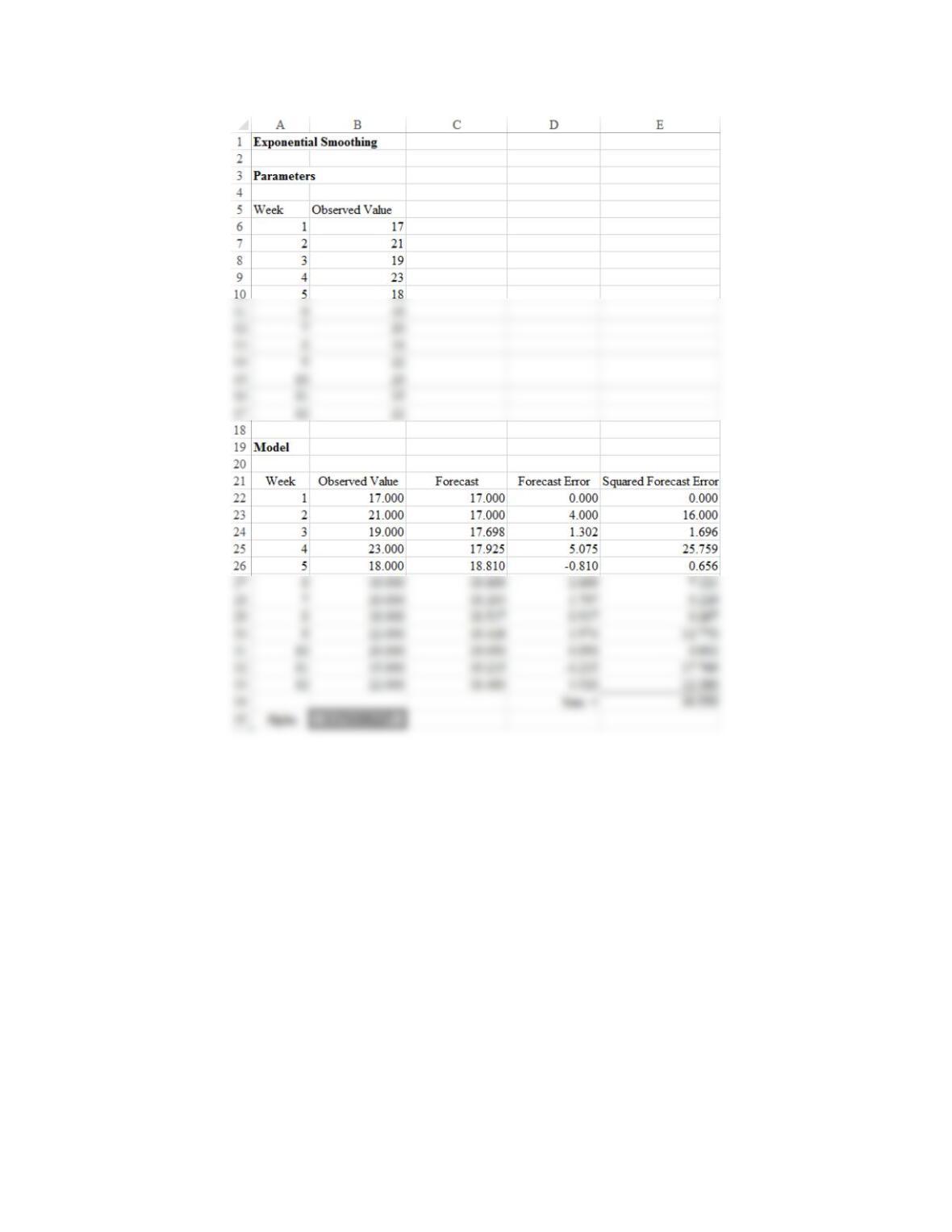
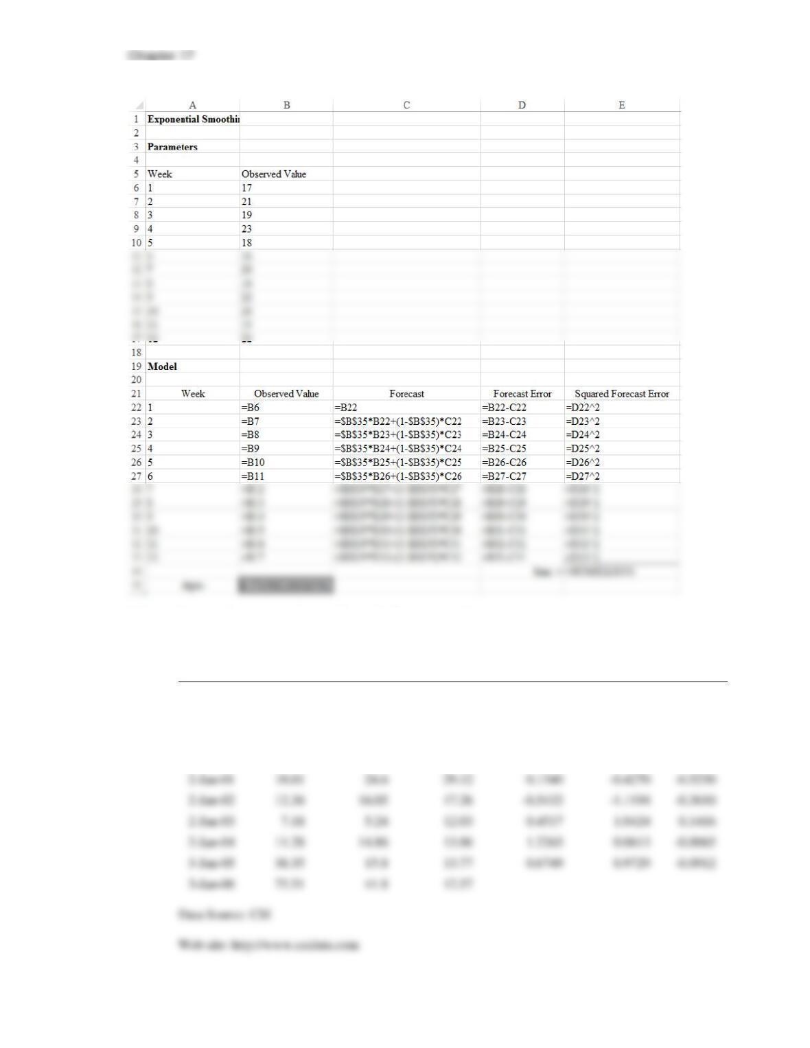
The optimal solution is
= 0.1744. The spreadsheet model follows.
Markov Processes
17 – 13
17 – 14
20. Here are the returns calculated from the Yahoo stock data.
AAPL
AMD
ORCL
AAPL
AMD
ORCL
Date
Adj. Close*
Adj. Close*
Adj. Close*
Return
Return
Return
2-Jan-97
4.16
17.57
4.32
0.0962
-0.5537
-0.1074
2-Jan-98
4.58
10.1
3.88
0.8104
0.1272
0.8666
4-Jan-99
10.30
11.47
9.23
0.9236
0.4506
0.9956
3-Jan-00
25.94
18
24.98
-0.8753
0.3124
0.1533
2-Jan-01
10.81
24.6
29.12
0.1340
-0.4270
-0.5230
2-Jan-02
12.36
16.05
17.26
-0.5432
-1.1194
-0.3610
2-Jan-03
7.18
5.24
12.03
0.4517
1.0424
0.1416
2-Jan-04
11.28
14.86
13.86
1.2263
0.0613
-0.0065
3-Jan-05
38.35
15.8
13.77
0.6749
0.9729
-0.0912
3-Jan-06
75.51
41.8
12.57
17 – 15
21. MODEL:
TITLE MARKOWITZ;
! SCENARIO 1 RETURN;
0.0962*AAPL – 0.5537*AMD – 0.1074*ORCL = R1;
! SCENARIO 2 RETURN;
0.8104*AAPL + 0.1272*AMD + 0.8666*ORCL = R2;
! SCENARIO 6 RETURN;
–0.5432*AAPL – 1.1194*AMD – 0.3610*ORCL = R6;
!SCENARIO 7 RETURN;
0.4517*AAPL + 1.0424*AMD + 0.1416*ORCL = R7;
!SCENARIO 8 RETURN;
1.2263*AAPL + 0.0613*AMD – 0.0065*ORCL = R8;
!SCENARIO 9 RETURN;
0.6749*AAPL + 0.9729*AMD – 0.0912*ORCL = R9;
@FREE(R1);
@FREE(R2);
@FREE(R3);
@FREE(R4);
@FREE(R5);
@FREE(R6);
@FREE(R7);
@FREE(R8);
@FREE(R9);
END
Chapter 17
17 – 16
Variable Value Reduced Cost
R1 –0.1457056 0.000000
RBAR 0.1518649 0.000000
R2 0.7316081 0.000000
R3 0.8905417 0.000000
R7 0.3499810 0.000000
R8 0.2290317 0.000000
R9 0.2276271 0.000000
AAPL 0.1817734 0.000000
22. MODEL:
TITLE MATCHING S&P INFO TECH RETURNS;
! MINIMIZE SUM OF SQUARED DEVIATIONS FROM S&P INFO TECH RETURNS;
MIN = ((R1 – .2854)^2 + (R2 – .7814)^2 + (R3 – .7874)^2 + (R4 +
.4090)^2 + (R5 + .2587)^2 + (R6 + .3741)^2 + (R7 – .4840)^2 +
(R8 – .0256)^2 + (R9 – 0.0099)^2);
! SCENARIO 1 RETURN;
! SCENARIO 5 RETURN;
0.1340*AAPL – 0.4270*AMD – 0.5230*ORCL = R5;
! SCENARIO 6 RETURN;
–0.5432*AAPL – 1.1194*AMD – 0.3610*ORCL = R6;
!SCENARIO 7 RETURN;
0.4517*AAPL + 1.0424*AMD + 0.1416*ORCL = R7;
!SCENARIO 8 RETURN;
1.2263*AAPL + 0.0613*AMD – 0.0065*ORCL = R8;
@FREE(R1);
@FREE(R2);
@FREE(R3);
@FREE(R4);
@FREE(R5);
@FREE(R6);
@FREE(R7);
@FREE(R8);
@FREE(R9);
END
17 – 17
R3 0.9716207 0.000000
R7 0.2353628 0.000000
R9 0.1328016 0.000000
AMD 0.6577707E–02 0.000000
23. In order to measure the semi-variance it is necessary to measure only the downside (deviation below
the mean). Do this by introducing two new variables for each scenario. For example, for scenario 1
define D1P as the deviation of return 1 above the mean, and D1N as the deviation of return 1 below
the mean. That is
11D P DIN R RBAR
− = −
45.42*FS – 1.33*IB + 41.46*LG + 7.06*LV + 58.68*SG + 5.43*SV = R4;
–21.93*FS + 7.36*IB – 23.26*LG – 5.37*LV – 9.02*SG + 17.31*SV = R5;
! INVESTMENT LEVELS SUM TO 1;
FS + IB + LG + LV + SG + SV = 1;
! DEFINE EXPECTED RETURN;
! MAKE THE RETURN VARIABLES UNRESTRICTED;
@FREE(R1);
@FREE(R2);
@FREE(R3);
Chapter 17
@FREE(R4);
@FREE(R5);
Local optimal solution found.
Objective value: 7.503540
Total solver iterations: 18
Model Title: MARKOWITZ WITH SEMIVARIANCE
Variable Value Reduced Cost
D1N 0.000000 0.000000
D2N 0.8595142 0.000000
D3N 3.412762 0.000000
LV 0.000000 14.14185
SG 0.8613837E–01 0.000000
SV 0.1589743 0.000000
R1 21.04766 0.000000
R2 9.140486 0.000000
R3 6.587238 0.000000
R4 7.656124 0.000000
R5 5.568495 0.000000
The solution calls for investing 69.1% of the portfolio in the intermediate-term bond fund, 6.4% of
the portfolio in the large-cap growth fund, 8.6% of the portfolio in the small-cap growth fund, and
15.9% of the portfolio in the small-cap value fund.
24. a. Let:
proportion of portfolio invested in the foreign stock mutual fund
proportion of portfolio invested in the intermediate-term bond fund
proportion of portfolio invested in the large-cap growth fu
FS
IB
LG
=
=
=nd
proportion of portfolio invested in the large-cap value fund
LV
=
17 – 19
1
2
3
Max
s.t.
10.06 17.64 32.41 32.36 33.44 24.56
13.12 3.25 18.71 20.61 19.40 25.32
13.47 7.51 33.28 12.93 3.85 6.70
45.42 1.33 41.46 7.06 58.68
R
FS IB LG LV SG SV R
FS IB LG LV SG SV R
FS IB LG LV SG SV R
FS IB LG LV SG
+ + + + + =
+ + + + + =
+ + + + − =
− + + + + 4
5.43
, , , , , 0
SV R
FS I B LG LV SG SV
=
b. The optimal solution is (% are rounded to one place):
Foreign Stick 13.3%
Intermediate-term Bond 49.6%
Large-Cap Growth 7.4%
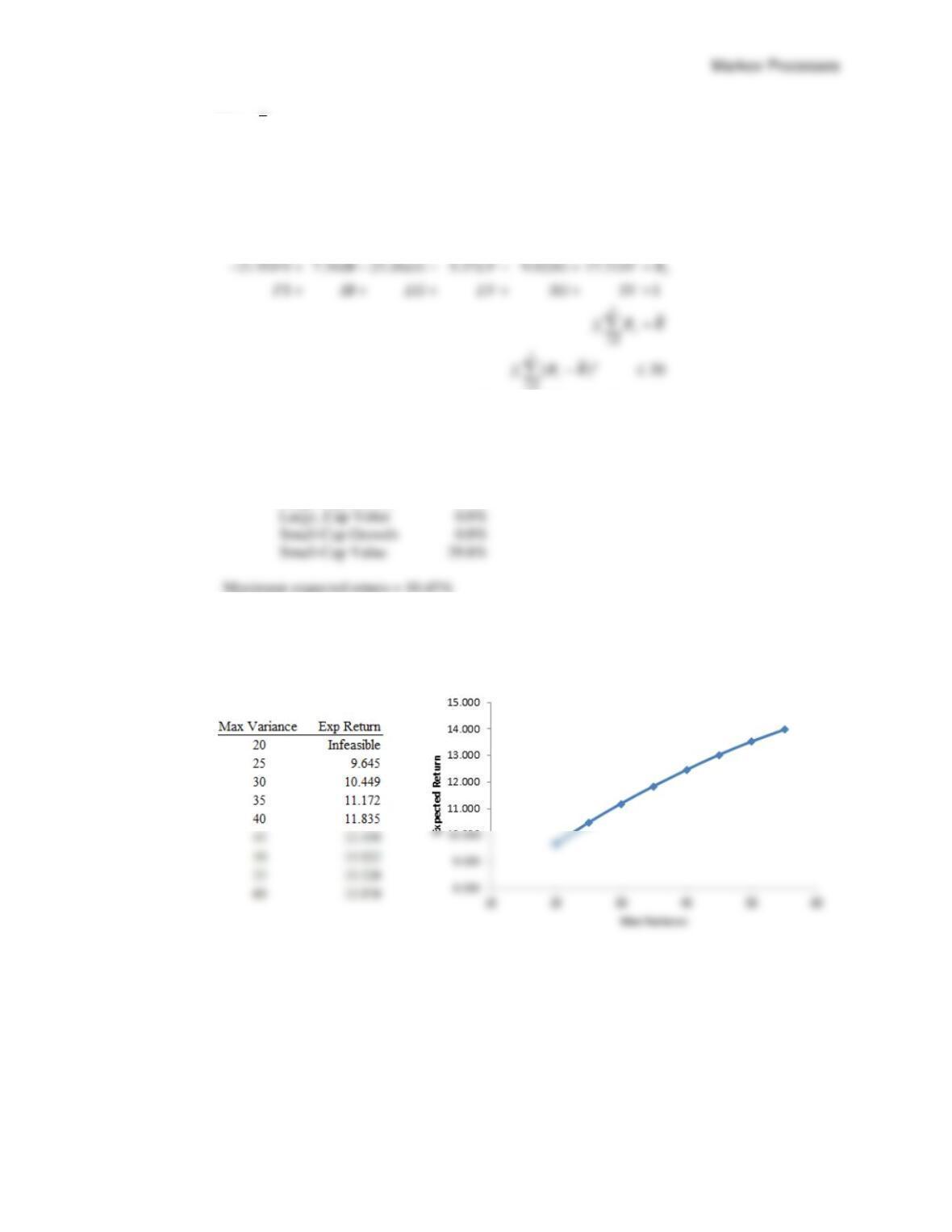
25. The efficient frontier is shown below. As the maximum variance increases the expected return
increases but at a decreasing rate.
26. This is a nonlinear 0/1 integer programming problem. Let XIJ = 1 if tanker I is assigned loading
dock J and 0 if not. First consider the constraints. Every tanker must be assigned to a loading dock.
These constraints are as follows.
! EACH TANKER MUST BE ASSIGNED A DOCK;
X11 + X12 + X13 = 1; !TANKER 1;
X21 + X22 + X23 = 1; !TANKER 2;
X31 + X32 + X33 = 1; !TANKER 3;
Chapter 17
Since there are three tankers and three loading docks each loading dock must be assigned to a tanker.
! EACH LOADING DOCK MUST BE ASSIGNED A TANKER;
The constraints that require each tanker to be assigned a loading dock, and each loading dock
assigned a tanker form the constraint set for the assignment problem. The assignment problem was
introduced in Chapter 6. However, unlike the assignment problem the objective function in this
problem is nonlinear. Consider, for example, the result of assigning tanker 1 to dock 2 and tanker 3
to dock 1. The distance between loading docks 1 and 2 is 100 meters. Also, tanker 1 must transfer
80 tons of goods to tanker 3. This means that 80 tons must be moved 100 meters. To capture this in
MIN = 100*60*X11*X22 + 150*60*X11*X23 + 100*80*X11*X32 +
150*80*X11*X33
+ 100*60*X12*X21 + 50*60*X12*X23 + 100*80*X12*X31 + 50*80*X12*X33
+ 150*60*X13*X21 + 50*60*X13*X22 + 150*80*X13*X31 + 50*80*X13*X32;
The solution to this model is
Global optimal solution found.
Objective value: 10000.00
Extended solver steps: 0
Total solver iterations: 38
Variable Value Reduced Cost
X11 0.000000 0.000000
X22 0.000000 0.000000
X23 0.000000 0.000000
X32 0.000000 0.000000
Thus tanker 1 should be assigned to dock 2, tanker 2 to dock 1 and tanker 3 to dock 3.
Depending on the starting point, Excel Solver will likely get stuck at a local optimum and not the
find the optimal solution that LINGO finds.
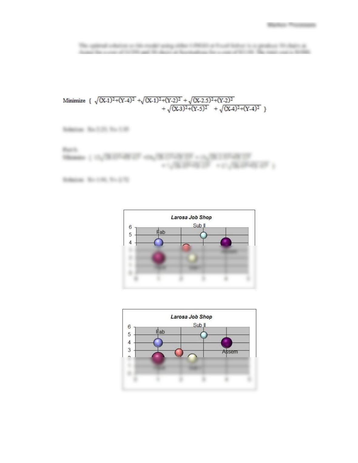
27. The objective is to minimize total production cost. To minimize total product cost minimize the
production cost at Aynor plus the production cost at Spartanburg. Minimize the production cost at
the two plants subject to the constraint that total production of kitchen chairs is equal to 40. The
model is:
17 – 21
28.
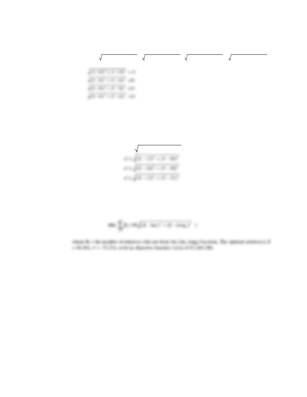
Part a.
Let X = the x coordinate of the tool bin
Y = the y coordinate of the tool bin
Part c.
Distance:
Demand-weighted Distance:
Using demand shifts the optimal location towards the paint cell (it has heavy demand).
Chapter 17
17 – 22
29. a. Let X = the horizontal coordinate of the tower.
Y = the vertical coordinate of the tower.
2 2 2 2 2 2 2 2
( ( 10) ( 10) ( 12) ( 16) ( 16) ( 18) ( 12) ( 22) )
..
Min X Y X Y X Y X Y
st
− + − + − + − + − + − + − + −
The optimal solution is X = 12, Y = 16, with an objective function value of 16.797.
b. Let d = the maximum distance and X and Y are as defined in part a.
22
..
( 10) ( 10)
Min d
st
d X Y
− + −
The optimal solution is X = 11.006 and Y = 15.999 with a maximum distance of 6.083.
30. Let X = the latitude of the optimal wedding location.
Y = the longitude of the optimal wedding location.