Markov Processes
17 – 1
Chapter 12
Advanced Optimization Applications
Learning Objectives
1. Learn about applications of more advanced optimization models that are solved in practice.
2. Develop an appreciation for the diversity of problems that can be modeled as optimization programs.
Note to Instructor
The application problems of Chapter 12 are designed to give the student an understanding and appreciation of
the broad range of problems that can be approached by optimization. The interpretation of the solution to
these problems will require the use of a software package such as Microsoft Excel‘s Solver or LINGO.
Chapter 17
17 – 2
Solutions:
1. a.
Min
E
s.t.
wg
+
wu
+
wc
+
ws
=
1
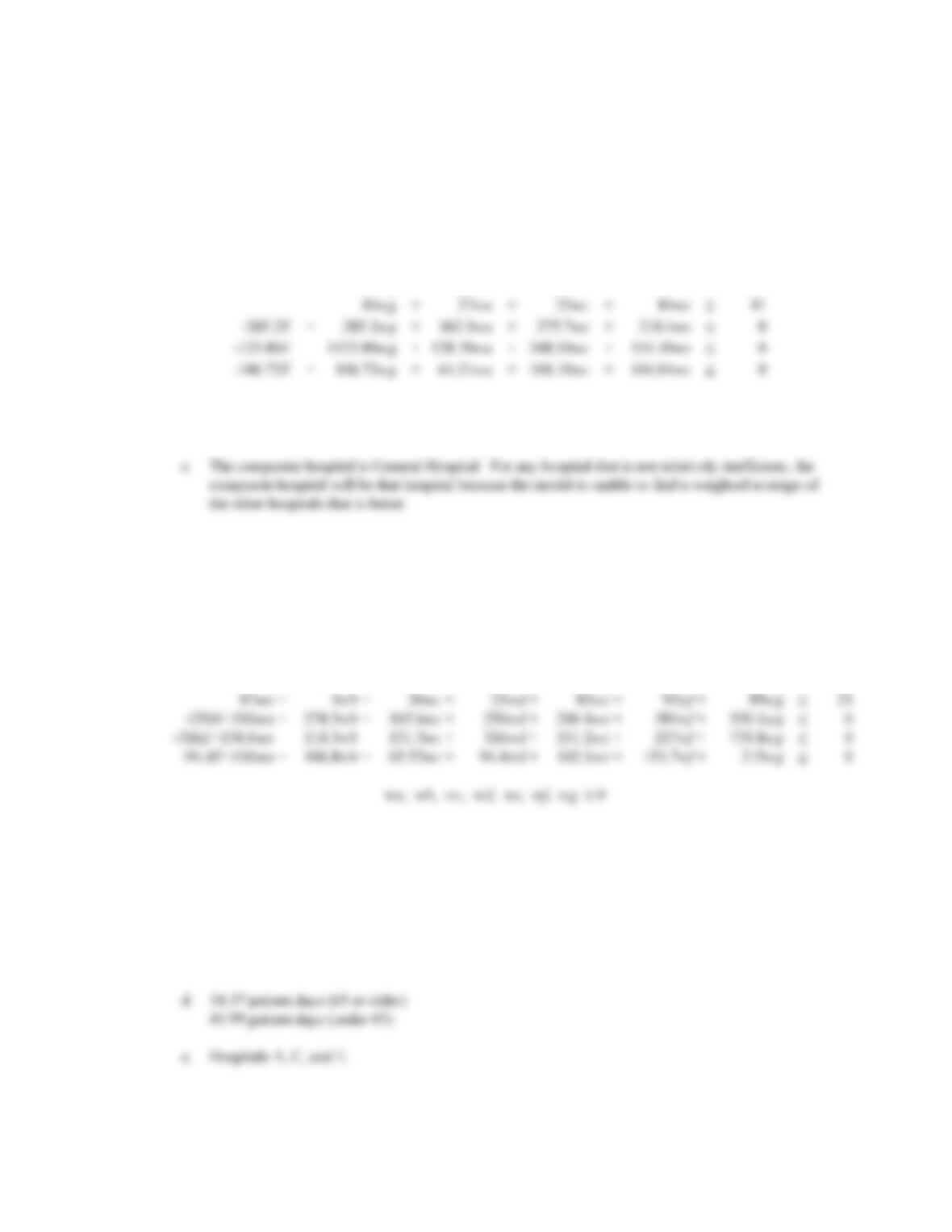
48.14wg
+
34.62wu
+
36.72wc
+
33.16ws
48.14
43.10wg
+
27.11wu
+
45.98wc
+
56.46ws
43.10
253wg
+
148wu
+
175wc
+
160ws
253
41wg
+
27wu
+
23wc
+
84ws
-285.2E
+
+
+
275.7wc
+
210.4ws
+
1123.80wg
+
+
+
154.10ws
+
+
64.21wu
+
+
wg, wu, wc, ws 0
b. Since wg = 1.0, the solution does not indicate General Hospital is relatively inefficient.
2. a.
Min E
s.t.
wa +
wb +
wc +
wd +
we +
wf +
wg
=
1
55.31wa +
37.64wb +
32.91wc +
33.53wd +
32.48we +
48.78wf +
58.41wg
33.53
49.52wa +
55.63wb +
25.77wc +
41.99wd +
55.30we +
81.92wf +
119.70wg
41.99
281wa +
156wb +
141wc +
160wd +
157we +
285wf +
111wg
160
47wa +
278.5wb +
165.6wc +
250wd +
206.4we +
114.3wb +
131.3wc +
316wd +
151.2we +
106.8wb +
65.52wc +
102.1we +
b. E = 0.924
wa = 0.074
wc = 0.436
we = 0.489
All other weights are zero.
c. D is relatively inefficient
Composite requires 92.4 of D‘s resources.
Markov Processes
17 – 3
4. a.
Min
E
s.t.
wb
+
wc
+
wj
+
wn
+
ws
=
1
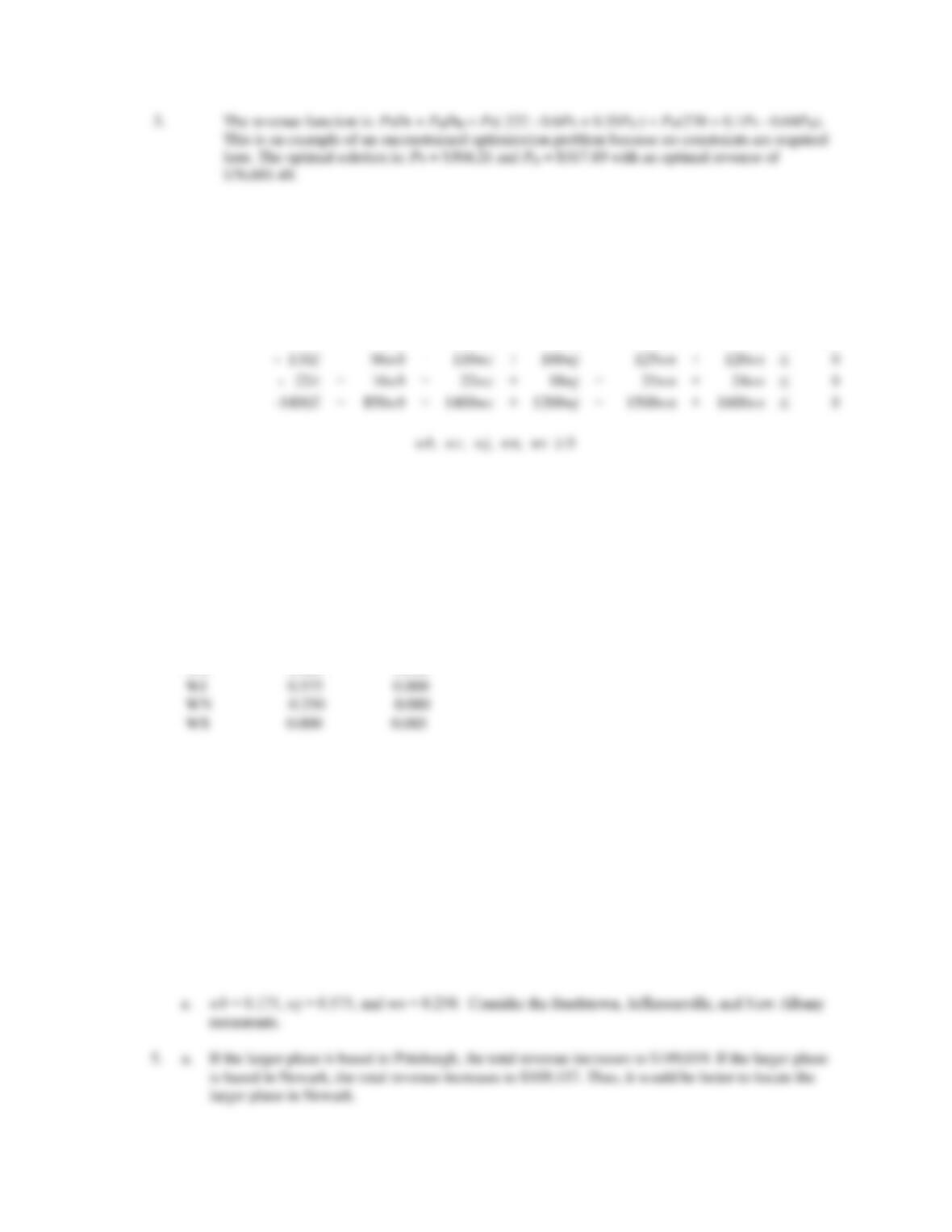
3800wb
+
4600wc
+
4400wj
+
6500wn
+
6000ws
4600
25wb
+
32wc
+
35wj
+
30wn
+
28ws
32
8wb
+
8.5wc
+
8wj
+
10wn
+
9ws
8.5
+
96wb
+
110wc
+
100wj
+
+
+
16wb
+
+
18wj
+
25wn
+
24ws
-1400E
+
+
1400wc
+
1200wj
+
1500wn
+
1600ws
b.
OPTIMAL SOLUTION
Objective Function Value = 0.960
Variable Value Reduced Costs
————– ————-— ——————
E 0.960 0.000
WB 0.175 0.000
c. Yes; E = 0.960 indicates a composite restaurant can produce Clarksville’s output with 96% of
Clarksville’s available resources.
d. More Output (Constraint 2 Surplus) $220 more profit per week.
Less Input
Hours of Operation 110E = 105.6 hours
FTE Staff 22E – 1.71 (Constraint 6 Slack) = 19.41
Supply Expense 1400E – 129.614 (Constraint 7 Slack) = $1214.39
The composite restaurant uses 4.4 hours less operation time, 2.6 less employees and $185.61 less
supplies expense when compared to the Clarksville restaurant.
Chapter 17
17 – 4
Note: The optimal solution to the original Leisure Air problem resulted in a total revenue of
$103,103. The difference between the total revenue for the original problem and the problem that
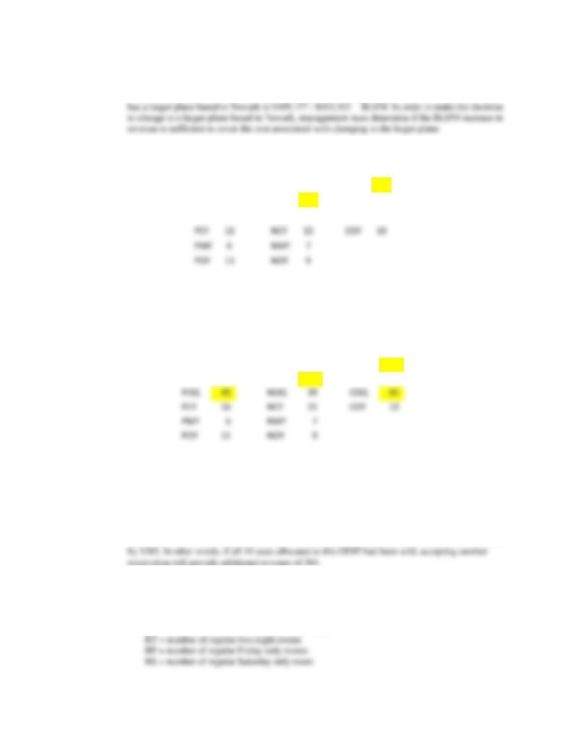
b. Using a larger plane based in Newark, the optimal allocations are:
PCQ
33
NCQ
26
CMQ
37
PMQ
44
NMQ
56
CMY
8
POQ
22
PCY
16
NCY
15
COY
10
PMY
NMY
POY
11
NOY
9
NOQ
39
COQ
41
The differences between the new allocations above and the allocations for the original Leisure Air
problem involve the two ODIFs that are highlighted in the solution shown above.
c. Using a larger plane based in Pittsburgh and a larger plane based in Newark, the optimal allocations
are:
PCQ
33
NCQ
26
CMQ
37
PMQ
44
NMQ
56
CMY
8
POQ
45
NOQ
39
COQ
44
PCY
16
NCY
15
COY
10
PMY
6
NMY
7
POY
11
NOY
The differences between the new allocations above and the allocations for the original Leisure Air
problem involve the four ODIFs that are boldfaced in the solution shown above. The total revenue
associated with the new optimal solution is $115,073, which is a difference of $115,073 – $103,103
= $11,970.
d. In part (b), the ODIF that has the largest bid price is NCY, with a bid price of $385. The bid price tells us
that if one more Y class seat were available from Newark to Charlotte that revenue would increase
6. The optimal solution is Q1 = 52.223, Q2 = 70.065, Q3 = 37.689 with a total cost of $25,830.
7. a. Let CT = number of convention two-night rooms
CF = number of convention Friday only rooms
CS = number of convention Saturday only rooms
Markov Processes
17 – 5

Chapter 17
17 – 6
b./c. The formulation and output are shown below.
LINEAR PROGRAMMING PROBLEM
MAX 225CT+123CF+130CS+295RT+146RF+152RS
S.T.
1) 1CT<40
2) 1CF<20
3) 1CS<15
4) 1RT<20
OPTIMAL SOLUTION
Objective Function Value = 25314.000
Variable Value Reduced Costs
————– ————— ——————
CT 36.000 0.000
CF 12.000 0.000
d. The shadow price for constraint 10 is 50 and shows an added profit of $50 if this additional
reservation is accepted.
8. To determine the percentage of the portfolio that will be invested in each of the mutual funds we use
the following decision variables:
FS = proportion of portfolio invested in a foreign stock mutual fund
IB = proportion of portfolio invested in an intermediate-term bond fund
17 – 7
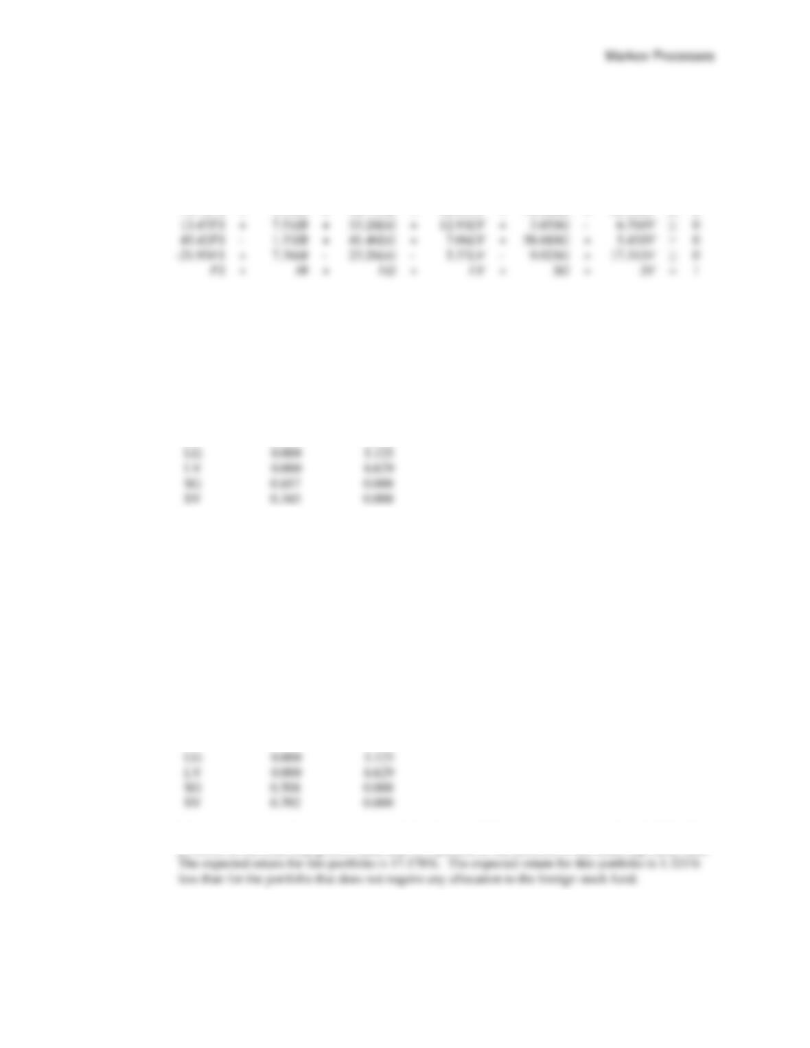
a. A portfolio model for investors willing to risk a return as low as 0% involves 6 variables and 6
constraints.
Max 12.03FS + 6.89IB + 20.52LG + 13.52LV + 21.27SG + 13.18SV
s.t.
10.06FS
+
17.64IB
+
32.41LG
+
32.36LV
+
33.44SG
+
24.56SV
≥
0
13.12FS
+
+
18.71LG
+
20.61LV
+
19.40SG
+
25.32SV
≥
0
13.47FS
+
+
33.28LG
+
12.93LV
+
–
≥
0
45.42FS
–
+
41.46LG
+
+
58.68SG
+
≥
0
+
–
23.26LG
–
–
+
17.31SV
≥
0
+
+
+
+
+
=
1
FS, IB, LG, LV, SG, SV ≥ 0
b. The solution obtained is shown.
Objective Function Value = 18.499
Variable Value Reduced Costs
————– ————— ——————
FS 0.000 13.207
IB 0.000 9.347
The recommended allocation is to invest 65.7% of the portfolio in a small-cap growth fund and
34.3% of the portfolio in a small-cap value fund. The expected return for this portfolio is 18.499%.
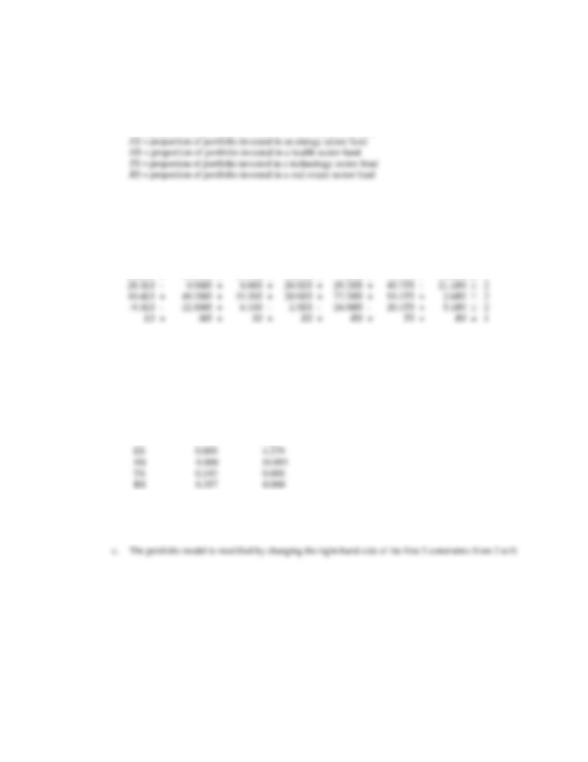
c. One constraint must be added to the model in part a. It is
FS ≥ .10
The solution is
Objective Function Value = 17.178
Variable Value Reduced Costs
————– ————— ——————
FS 0.100 0.000
IB 0.000 9.347
The recommended allocation is to invest 10% of the portfolio in the foreign stock fund, 50.8% of the
Chapter 17
17 – 8
9. To determine the percentage of the portfolio that will be invested in each of the mutual funds we use
the following decision variables:
LS = proportion of portfolio invested in a large-cap stock mutual fund
MS = proportion of portfolio invested in a mid-cap stock fund
SS = proportion of portfolio invested in a small-cap growth fund
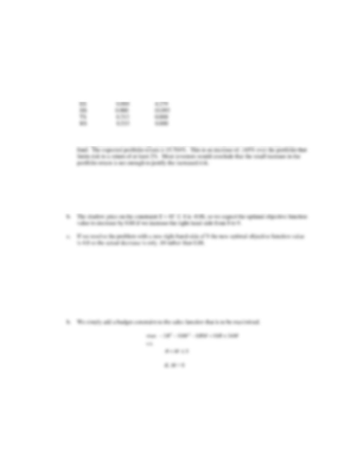
a. A portfolio model for investors willing to risk a return as low as 0% involves 7 variables and 6
constraints.
Max 9.68LS + 5.91MS + 15.20SS + 11.74ES + 7.34HS + 16.97TS + 15.44RS
s.t.
35.3LS
+
32.3MS
+
20.8SS
+
25.3ES
+
49.1HS
+
46.2TS
+
20.5RS
≥
2
20.0LS
+
23.2MS
+
22.5SS
+
33.9ES
+
5.5HS
+
21.7TS
+
44.0RS
≥
2
28.3LS
–
+
+
20.5ES
+
29.7HS
+
45.7TS
–
21.1RS
≥
2
10.4LS
+
49.3MS
+
33.3SS
+
20.9ES
+
77.7HS
+
93.1TS
+
≥
2
–
22.8MS
+
–
–
24.9HS
–
20.1TS
+
≥
2
+
+
+
+
+
+
=
1
LS, MS, SS, ES, HS, TS, RS ≥ 0
b. The solution obtained is:
Objective Function Value = 15.539
Variable Value Reduced Costs
————– ————— ——————
LS 0.000 6.567
MS 0.000 11.548
SS 0.500 0.000
The recommended allocation is to invest 50% of the portfolio in the small-cap stock fund, 14.3% of
the portfolio in the technology sector fund, and 35.7% of the portfolio in the real estate sector fund.
The expected portfolio return is 15.539%.
Markov Processes
17 – 9
d. The solution obtained is:
Objective Function Value = 15.704
Variable Value Reduced Costs
————– ————— ——————
LS 0.000 6.567
MS 0.000 11.548
SS 0.255 0.000
The recommended allocation is to invest 25.5% of the portfolio is the small-cap stock fund, 21.2%
10. Using LINGO or Excel Solver, the optimal solution is X = 2, Y = -4, for an optimal solution value
of 0.
11. a. Using LINGO or Excel Solver, the optimal solution is X = 4.32, Y = 0.92, for an optimal solution
value of 4.84
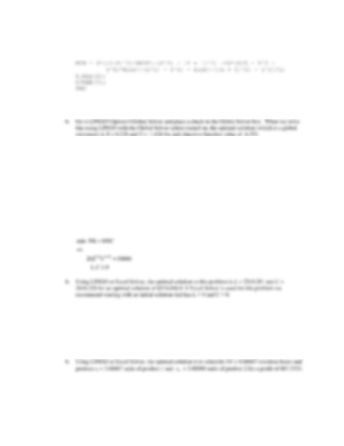
12. a. With $1000 being spent on radio and $1000 being spent on direct mail we can simply substitute
those values into the sales function.
S = -2R2 – 10 M2 – 8RM + 18R + 34M
= -2(22) – 10(12) – 8(2)(1) + 18(2) + 34(1)
= –8 – 10 – 16 + 36 + 34
= 36
Sales of $36,000 will be realized with this allocation of the media budget.
c. Using LINGO or Excel Solver, we find that the optimal solution is to invest $2,500 in radio
advertising and $500 in direct mail advertising. The total sales generated will be $37,000.
Chapter 17
17 – 10
13. a. Here is the proper LINGO formulation. Note the extra use of parentheses needed because of the way
LINGO uses the unary minus sign. For example, –X^2 is written as –(X^2)
Minimizing this function without the global solver option turned on in LINGO gives X = 4.978 and
Y = 1.402 for a value of 0.3088137E-08. This is a local minimum.
14. a. The optimization model is
.25 .75
Max 5
s.t.
25 75 75000
,0
LC
LC
LC
+
b. Using LINGO or Excel Solver, the optimal solution to this is L = 750 and C = 750 for an optimal
objective function value of 3750. If Excel Solver is used for this problem we recommend starting
with an initial solution that has L > 0 and C > 0.
15. a. The optimization model is
16. a. Let OT be the number of overtime hours scheduled. Then the optimization model is
22
1 1 2 2
12
12
max 3 42 3 48 700 5
. .
4 6 24
, , 0
x x x x OT
st
x x OT
x x OT
− + − + + −
+ +
17 – 11
17. a. If X is the weekly production volume in thousand of units at the Dayton plant and Y is the weekly
production volume in thousands of units at the Hamilton plant, then the optimization model is
18.
MODEL:
TITLE MARKOWITZ;
! MINIMIZE VARIANCE OF THE PORTFOLIO;
MIN = (1/5)*((R1 – RBAR)^2 + (R2 – RBAR)^2 + (R3 – RBAR)^2 + (R4 –
RBAR)^2 + (R5 – RBAR)^2);
! SCENARIO 4 RETURN;
45.42*FS – 1.33*IB + 41.46*LG + 7.06*LV + 58.68*SG + 5.43*SV = R4;
! SCENARIO 5 RETURN;
–21.93*FS + 7.36*IB – 23.26*LG – 5.37*LV – 9.02*SG + 17.31*SV = R5;
! MUST BE FULLY INVESTED IN THE MUTUAL FUNDS;
FS + IB + LG + LV + SG + SV = 1;
! SCENARIO RETURNS MAY BE NEGATIVE;
@FREE(R1);
@FREE(R2);
@FREE(R3);
@FREE(R4);
@FREE(R5);
END
Local optimal solution found.
Objective value: 27.13615
Total solver iterations: 17