
Page 16 of 30
12.
b. Is the process in control? Explain.
The process is not in control.
Experiment: Randomly select the heights of at least 15 of the students in your class.
a. Develop a control chart and plot the heights on the chart.
b. Which chart should you use?
c. Is this process in control?
Results will vary.
13.
A finishing process packages assemblies into boxes. You have noticed variability in
the boxes and desire to improve the process to fix the problem because some products
fit too tightly into the boxes and others fit too loosely.
Following are width measurements for the boxes.
Sample
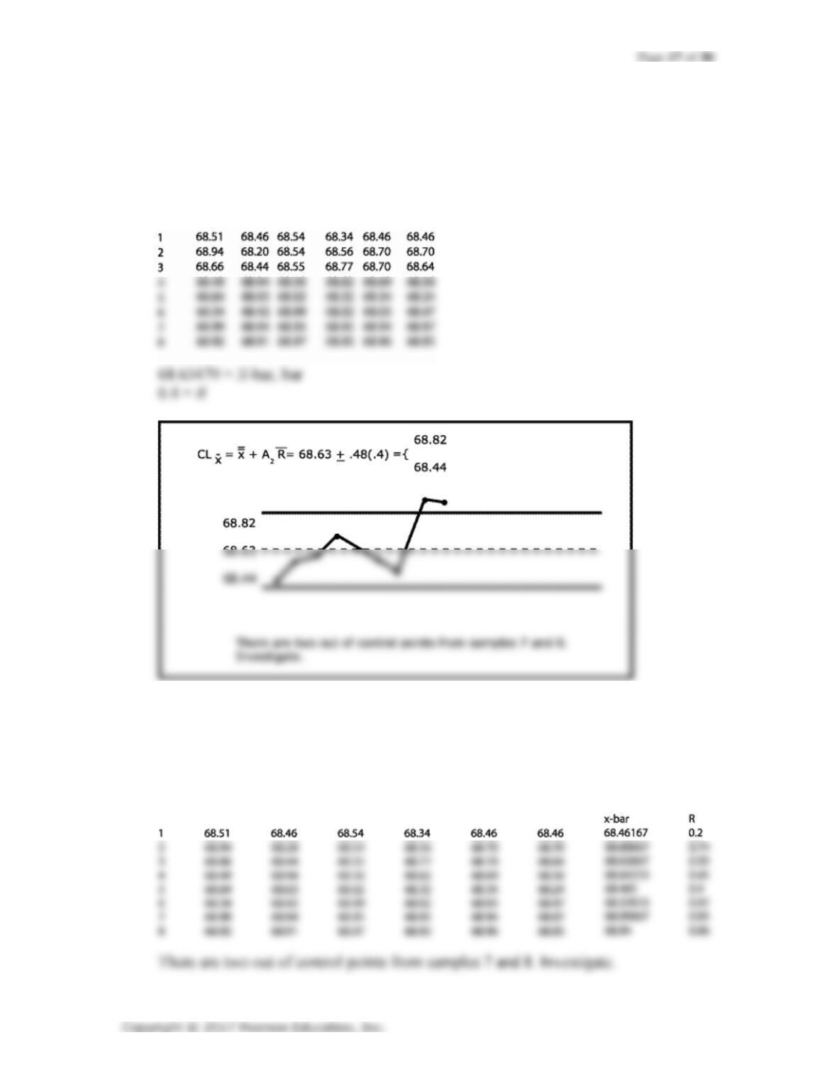
Using x-bar and R charts, plot and interpret the process.
Answer:
x-bar and R chart computations:
Page 18 of 30
14.
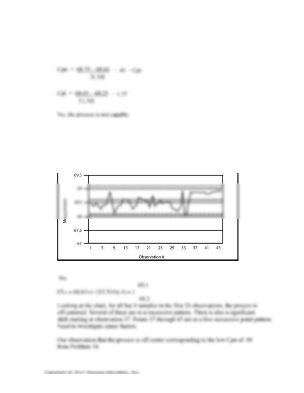
For the data in problem 13, if the mean specification is 68.5 +/- .25 and the estimated
process standard deviation is .10, is the process capable? Compute Cpu, Cpl, and Cpk.
15.
For the data in problem 13, treat the data as if it were population data, and find the
limits for an x-bar chart. Is the process in control? Compare your answer with the answers to Prob
Hint: Use the formula CLx = x-bar (3/d2)R-bar (Figure 11-8)
36.012
48.6
50.28
64.548
2
52
45
54
75
64
58
30
3
34
64
36
46
63
48.6
30
4
34
45
47
37
62
45
13
5
46
64
75
55
16
51.2
29
Grand
Mean:
50.28
D3 = 0
CL x-bar = 50.28 +/– .58(24.6) = (64.548; 36.012)
LCL R =
0
UCL R = 2.11*24.6 = 51.906
36.012
51.2
50.28
64.548
16.
A Rochester, NY firm produces grommets that have to fit into a slot in an assembly.
Following are dimensions of grommets (in millimeters):
Sample
x
1
46
33
54
46
64
2
52
45
54
75
64
3
34
64
36
46
63
4
34
45
47
37
62
5
46
64
75
55
16
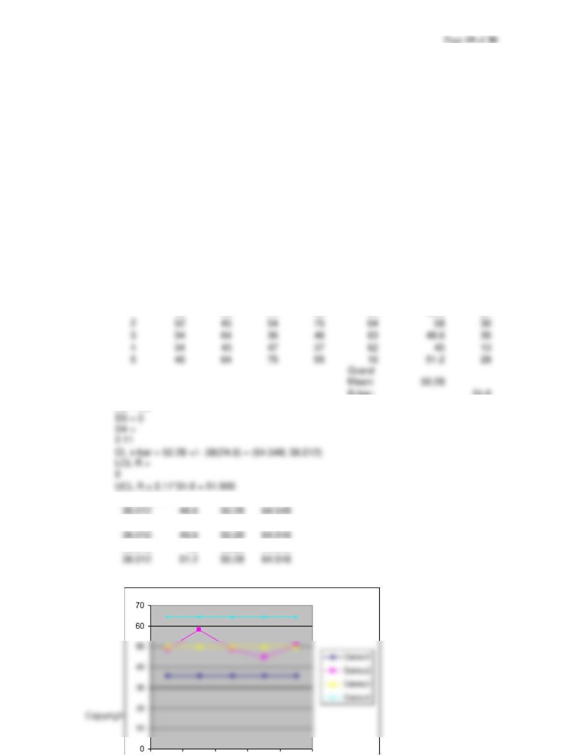
a. Use x-bar and R charts to determine if the process is in control.
Sample
x
Means
Ranges
1
46
33
54
46
64
48.6
21
R-bar:
24.6
A2 = .58
X-bar Chart:
36.012
58
50.28
64.548
36.012
48.6
50.28
64.548
36.012
45
50.28
64.548
Page 20 of 30
68.51
68.94
68.66
68.49
68.64
68.34
68.99
68.92
0
30
24.6
51.906
0
13
24.6
51.906
0
29
24.6
51.906
17.
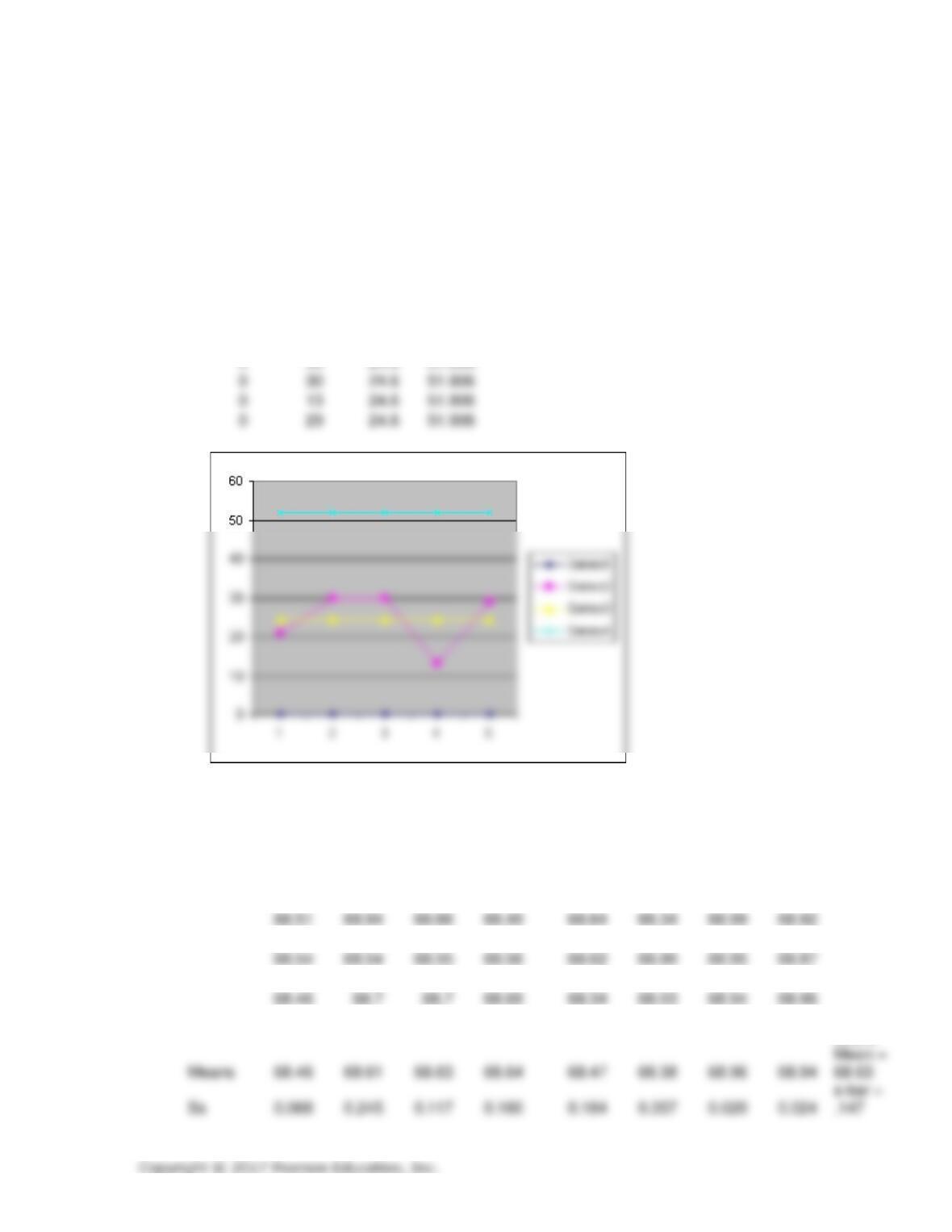
R-Chart
0
21
24.6
51.906
0
30
24.6
51.906
The process is in control.
Using the data from Problem 13, compute the limits for x-bar and s charts. Is the
process still in control?
Sample
1
2
3
4
5
6
7
8
68.46
68.2
68.44
68.94
68.63
68.42
68.94
68.91
68.54
68.54
68.55
68.56
68.62
68.99
68.95
68.97
68.34
68.56
68.77
68.62
68.32
68.02
68.95
68.93
68.46
68.7
68.7
68.69
68.34
68.03
68.94
68.96
68.46
68.7
68.64
68.56
68.24
68.47
68.97
68.95
Grand
Page 21 of 30
68.44
68.462
68.635
68.82
68.44
68.627
68.635
68.82
68.44
68.465
68.635
68.82
0.00441
0.16
0.147
0.2896
0.00441
0.357
0.147
0.2896
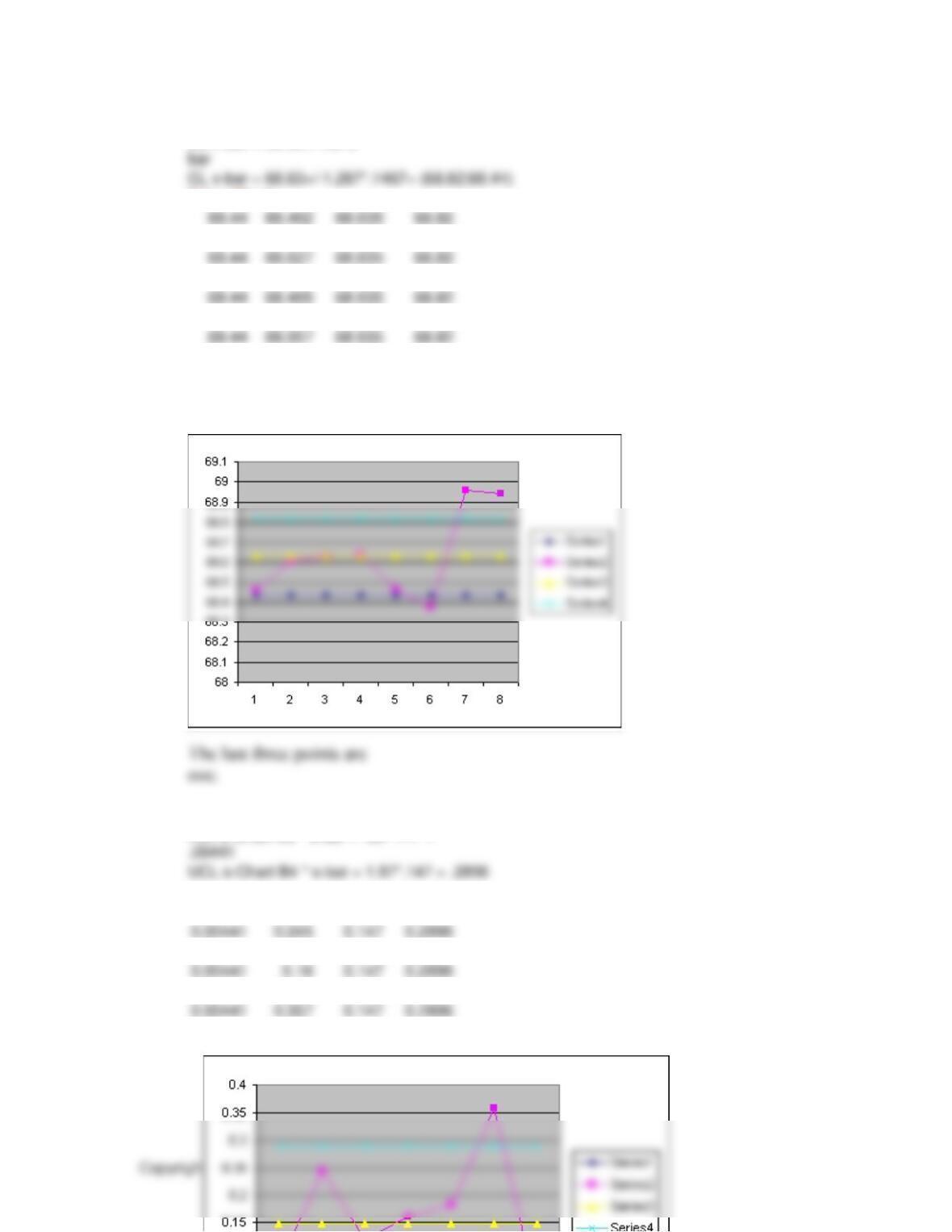
CL x-bar = 68.63+/-1.287*.1467= (68.82;68.44)
.00441
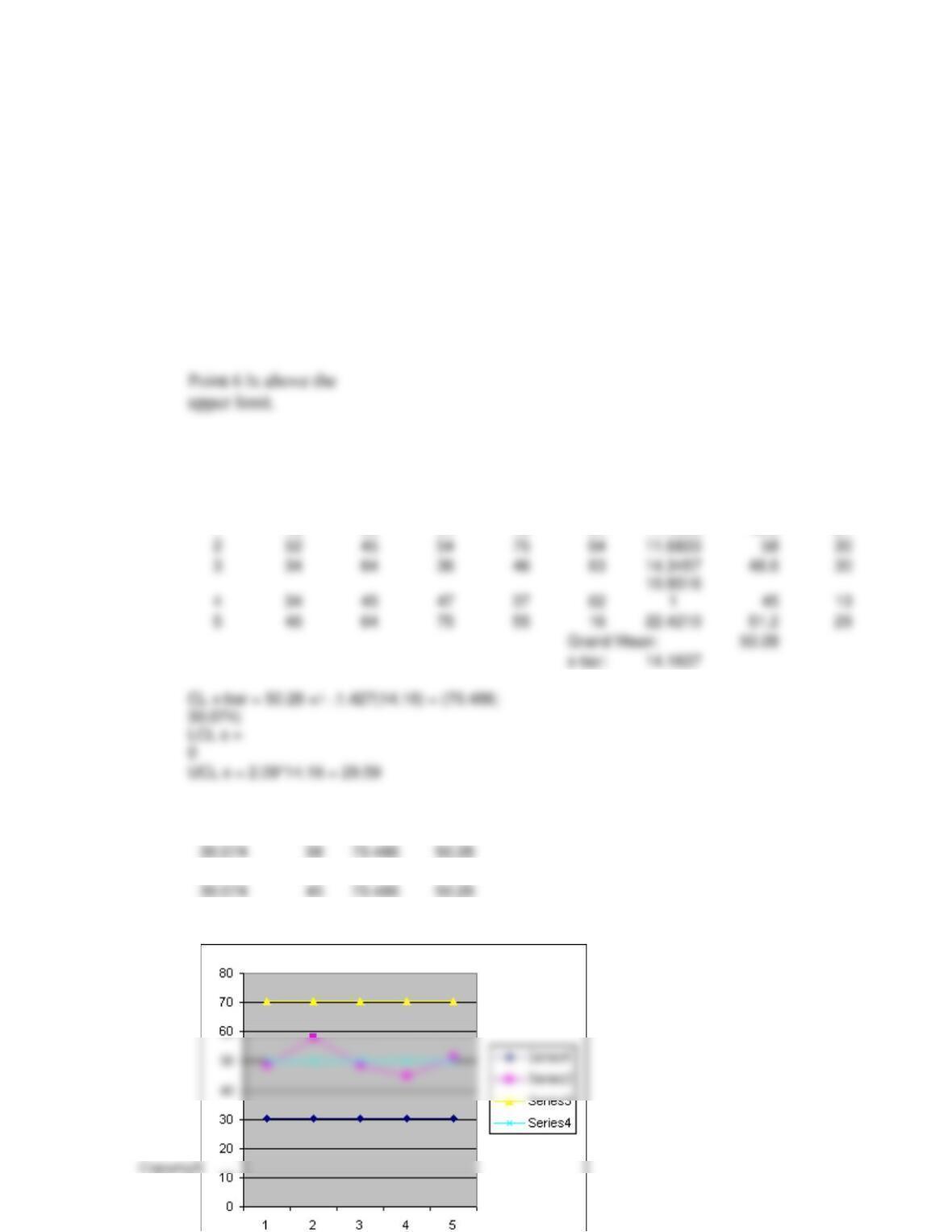
UCL s-Chart B4 * s-bar = 1.97*.147 = .2896
n=6
CL x-bar = 68.63+/-A3*s-
X-bar Chart
68.44
68.607
68.635
68.82
68.44
68.643
68.635
68.82
68.44
68.378
68.635
68.82
68.44
68.957
68.635
68.82
68.44
68.94
68.635
68.82
s-Chart
LCL s-Chart B3 * s-bar = .03*.147 =
0.00441
0.068
0.147
0.2896
0.00441
0.245
0.147
0.2896
0.00441
0.117
0.147
0.2896
0.00441
0.184
0.147
0.2896
0.00441
0.02
0.147
0.2896
Page 22 of 30
2
52
45
54
75
64
11.6833
30
3
34
64
36
46
63
14.3457
48.6
30
4
34
45
47
37
62
1
13
5
46
64
75
55
16
22.4210
51.2
29
Grand Mean:
s-bar:
14.1637
30.074)
0
UCL s = 2.09*14.16 = 29.59
18.
Using the data from Problem 16, compute the limits for x-bar and s charts. Is the process
still in control?
Sample
x
Std Dev
Means
Ranges
1
46
33
54
46
64
11.4368
48.6
21
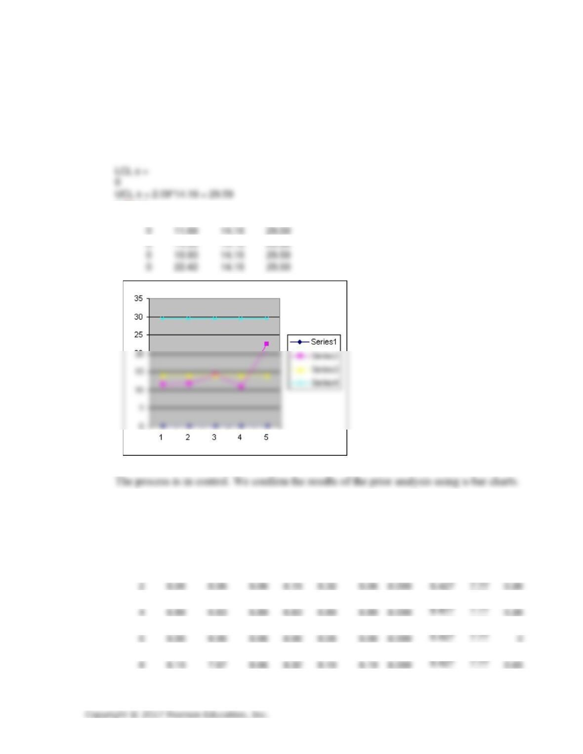
x-bar Chart
30.074
48.6
70.486
50.28
30.074
70.486
50.28
30.074
48.6
70.486
50.28
30.074
70.486
50.28
30.074
51.2
70.486
50.28
Page 23 of 30
UCL s = 2.09*14.16 = 29.59
0
14.35
14.16
29.59
0
10.93
14.16
29.59
0
22.42
14.16
29.59
19.
s Chart
0
11.44
14.16
29.59
0
11.68
14.16
29.59
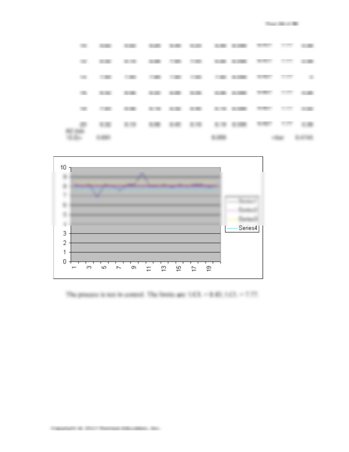
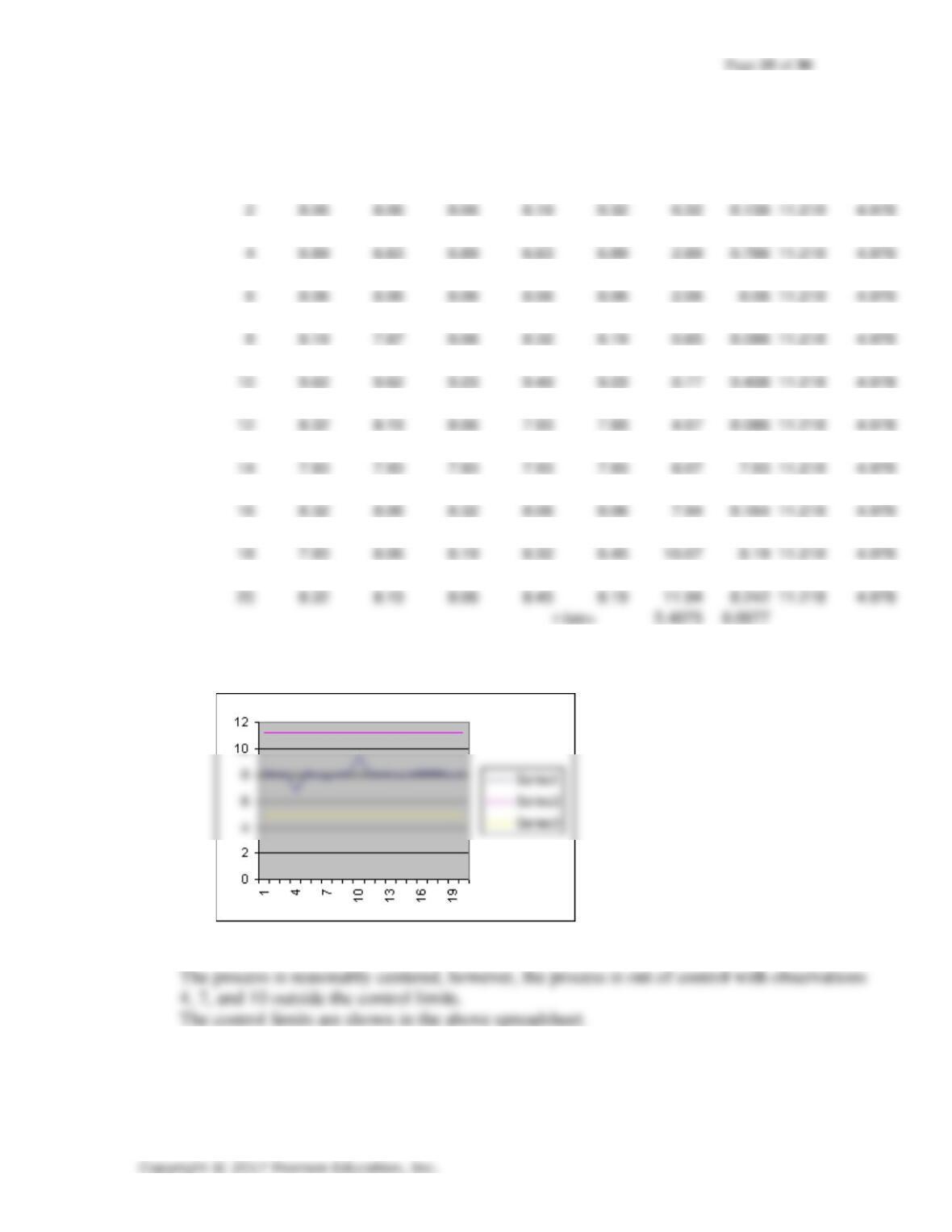
Use a median chart to determine if this process is centered.
See the Excel spreadsheet below. Data from the textbook has been entered.
Sample
Medians
CL
UCL
LCL
Ranges
1
8.06
7.93
8.19
8.45
8.32
8.19
8.099
8.427
7.77
0.52
2
8.06
8.06
8.06
8.19
8.32
8.06
8.099
8.427
7.77
0.26
3
8.19
7.67
8.06
8.32
8.19
8.19
8.099
8.427
7.77
0.65
4
6.89
6.63
6.89
6.63
6.89
6.89
8.099
8.427
7.77
0.26
5
7.93
8.58
8.19
8.06
8.32
8.19
8.099
8.427
7.77
0.65
6
8.06
8.06
8.06
8.06
8.06
8.06
8.099
8.427
7.77
0
7
7.54
7.41
7.67
9.36
6.76
7.54
8.099
8.427
7.77
2.6
8
8.19
7.67
8.06
8.32
8.19
8.19
8.099
8.427
7.77
0.65
9
8.19
7.67
8.06
8.32
8.19
8.19
8.099
8.427
7.77
0.65
11
8.06
8.19
8.06
8.19
8.06
8.06
8.099
8.427
7.77
0.13
12
8.32
8.19
8.06
7.93
7.93
8.06
8.099
8.427
7.77
0.39
13
8.19
8.32
8.06
8.19
7.93
8.19
8.099
8.427
7.77
0.39
14
7.93
7.93
7.93
7.93
7.93
7.93
8.099
8.427
7.77
15
8.19
8.32
7.93
8.19
7.93
8.19
8.099
8.427
7.77
0.39
16
8.32
8.06
8.32
8.06
8.06
8.06
8.099
8.427
7.77
0.26
17
8.06
8.32
8.19
8.32
8.06
8.19
8.099
8.427
7.77
0.26
18
7.93
8.06
8.19
8.32
8.45
8.19
8.099
8.427
7.77
0.52
19
8.06
7.93
7.93
7.93
7.93
7.93
8.099
8.427
7.77
0.13
20
8.32
8.19
8.06
8.45
8.19
8.19
8.099
8.427
7.77
0.39
20.
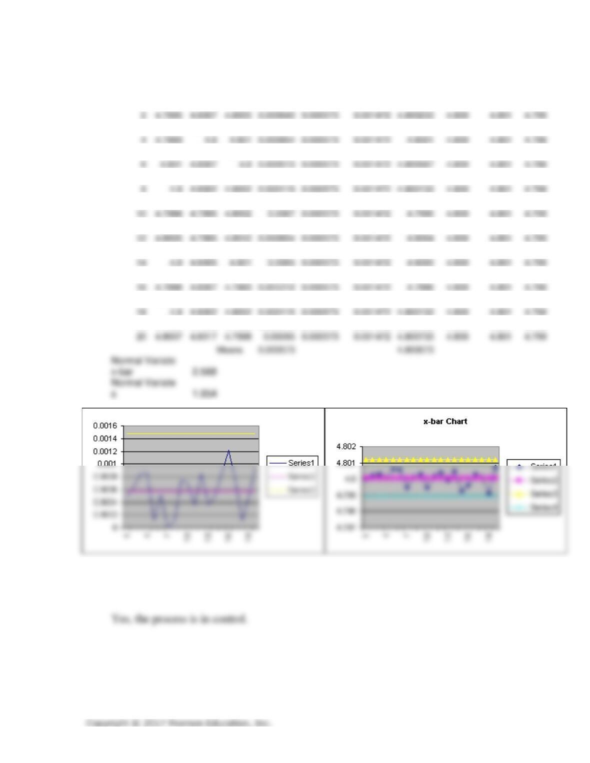
Use an x-bar chart to determine if the data in Problem 19 are in control.
Do you get the same answer?
Sample
ranges
means
ucl
lcl
1
8.06
7.93
8.19
8.45
8.32
7.45
8.19
11.218
4.978
2
8.06
8.06
8.06
8.19
8.32
6.32
8.138
11.218
4.978
3
8.19
7.67
8.06
8.32
8.19
5.32
8.086
11.218
4.978
4
6.89
6.63
6.89
6.63
6.89
2.89
6.786
11.218
4.978
5
7.93
8.58
8.19
8.06
8.32
3.58
8.216
11.218
4.978
6
8.06
8.06
8.06
8.06
8.06
2.06
8.06
11.218
4.978
7
7.54
7.41
7.67
9.36
6.76
2.6
7.748
11.218
4.978
8
8.19
7.67
8.06
8.32
8.19
0.65
8.086
11.218
4.978
9
8.19
7.67
8.06
8.32
8.19
1.33
8.086
11.218
4.978
11
8.06
8.19
8.06
8.19
8.06
2.94
8.112
11.218
4.978
12
8.32
8.19
8.06
7.93
7.93
4.07
8.086
11.218
4.978
13
8.19
8.32
8.06
8.19
7.93
5.07
8.138
11.218
4.978
14
7.93
7.93
7.93
7.93
7.93
6.07
7.93
11.218
4.978
15
8.19
8.32
7.93
8.19
7.93
7.07
8.112
11.218
4.978
16
8.32
8.06
8.32
8.06
8.06
7.94
8.164
11.218
4.978
17
8.06
8.32
8.19
8.32
8.06
8.94
8.19
11.218
4.978
18
7.93
8.06
8.19
8.32
8.45
10.07
8.19
11.218
4.978
19
8.06
7.93
7.93
7.93
7.93
11.07
7.956
11.218
4.978
20
8.32
8.19
8.06
8.45
8.19
11.94
8.242
11.218
4.978
r-bar=
5.4075
a2=
0.577
21.
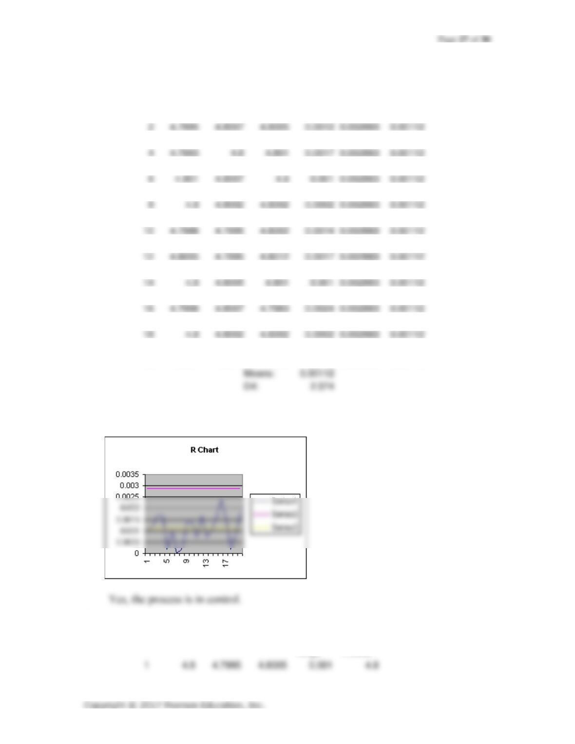
The following data are for a component used in the space shuttle. Since the process
dispersion is closely monitored, use an x-bar and s chart to see if the process is in
control.
Page 26 of 30
Sample
St devs
cls
Ucls
x-bar
clx-bar
ucl x-bar
lcl x-bar
1
4.8
4.7995
4.8005
0.0005
0.000573
0.001472
4.8
4.800
4.801
4.799
2
4.7995
4.8007
4.8005
0.000643
0.000573
0.001472
4.800233
4.800
4.801
4.799
3
4.7995
4.8002
4.8012
0.000854
0.000573
0.001472
4.8003
4.800
4.801
4.799
4
4.7993
4.8
4.801
0.000854
0.000573
0.001472
4.8001
4.800
4.801
4.799
5
4.8007
4.8007
4.8005
0.000115
0.000573
0.001472
4.800633
4.800
4.801
4.799
6
4.801
4.8007
4.8
0.000513
0.000573
0.001472
4.800567
4.800
4.801
4.799
7
4.7995
4.7995
4.7995
0
0.000573
0.001472
4.7995
4.800
4.801
4.799
8
4.8
4.8002
4.8002
0.000115
0.000573
0.001472
4.800133
4.800
4.801
4.799
9
4.8012
4.8
4.7998
0.000757
0.000573
0.001472
4.800333
4.800
4.801
4.799
10
4.7988
4.7995
4.8002
0.0007
0.000573
0.001472
4.7995
4.800
4.801
4.799
11
4.8005
4.7998
4.8002
0.000351
0.000573
0.001472
4.800167
4.800
4.801
4.799
13
4.8
4.8002
4.7995
0.000361
0.000573
0.001472
4.7999
4.800
4.801
4.799
14
4.8
4.8005
4.801
0.0005
0.000573
0.001472
4.8005
4.800
4.801
4.799
15
4.7986
4.8002
4.799
0.000833
0.000573
0.001472
4.799267
4.800
4.801
4.799
16
4.7998
4.8007
4.7983
0.001212
0.000573
0.001472
4.7996
4.800
4.801
4.799
17
4.8005
4.7995
4.801
0.000764
0.000573
0.001472
4.800333
4.800
4.801
4.799
18
4.8
4.8002
4.8002
0.000115
0.000573
0.001472
4.800133
4.800
4.801
4.799
19
4.7993
4.7986
4.7995
0.000473
0.000573
0.001472
4.799133
4.800
4.801
4.799
20
4.8007
4.8017
4.7998
0.000573
0.001472
4.800733
4.800
4.801
4.799
Means
0.000573
4.800073
2
4.7995
4.8007
4.8005
0.0012
0.002883
0.00112
4
4.7993
4.8
4.801
0.0017
0.002883
0.00112
6
4.801
4.8007
4.8
0.001
0.002883
0.00112
8
4.8
4.8002
4.8002
0.0002
0.002883
0.00112
12
4.8005
4.7995
4.8012
0.0017
0.002883
0.00112
14
4.8
4.8005
4.801
0.001
0.002883
0.00112
16
4.7998
4.8007
4.7983
0.0024
0.002883
0.00112
18
4.8
4.8002
4.8002
0.0002
0.002883
0.00112
Means:
0.00112
D4:
2.574
22.
23.
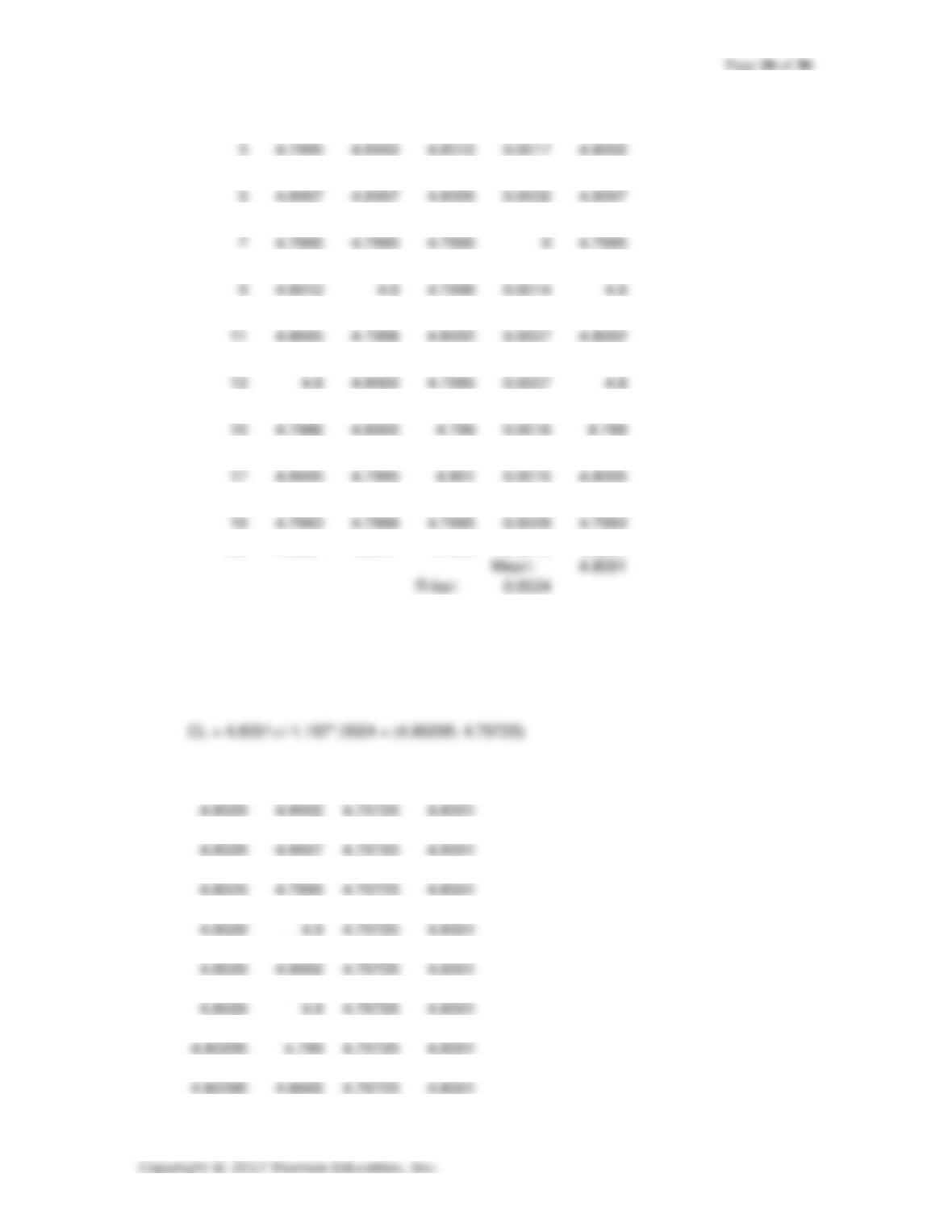
Develop an R-chart for the data in Problem 21. Do you get the same answer?
Sample
Ranges
UCLs
CLs
1
4.8
4.7995
4.8005
0.001
0.002883
0.00112
3
4.7995
4.8002
4.8012
0.0017
0.002883
0.00112
5
4.8007
4.8007
4.8005
0.0002
0.002883
0.00112
7
4.7995
4.7995
4.7995
0
0.002883
0.00112
9
4.8012
4.8
4.7998
0.0014
0.002883
0.00112
11
4.8005
4.7998
4.8002
0.0007
0.002883
0.00112
13
4.8
4.8002
4.7995
0.0007
0.002883
0.00112
15
4.7986
4.8002
4.799
0.0016
0.002883
0.00112
17
4.8005
4.7995
4.801
0.0015
0.002883
0.00112
19
4.7993
4.7986
4.7995
0.0009
0.002883
0.00112
20
4.8007
4.8017
4.7998
0.0019
0.002883
0.00112
Using the data from Problem 21, compute limits for a median chart. Is the process
in control?
range
median
3
4.7995
4.8002
4.8012
0.0017
4.8002
5
4.8007
4.8007
4.8005
0.0002
4.8007
7
4.7995
4.7995
4.7995
0
4.7995
15
4.7986
4.8002
4.799
0.0016
4.799
17
4.8005
4.7995
4.801
0.0015
4.8005
4.8029
4.8002
4.79725
4.8001
4.8029
4.8
4.79725
4.8001
4.8029
4.8002
4.79725
4.8001
4.8029
4.8
4.79725
4.8001
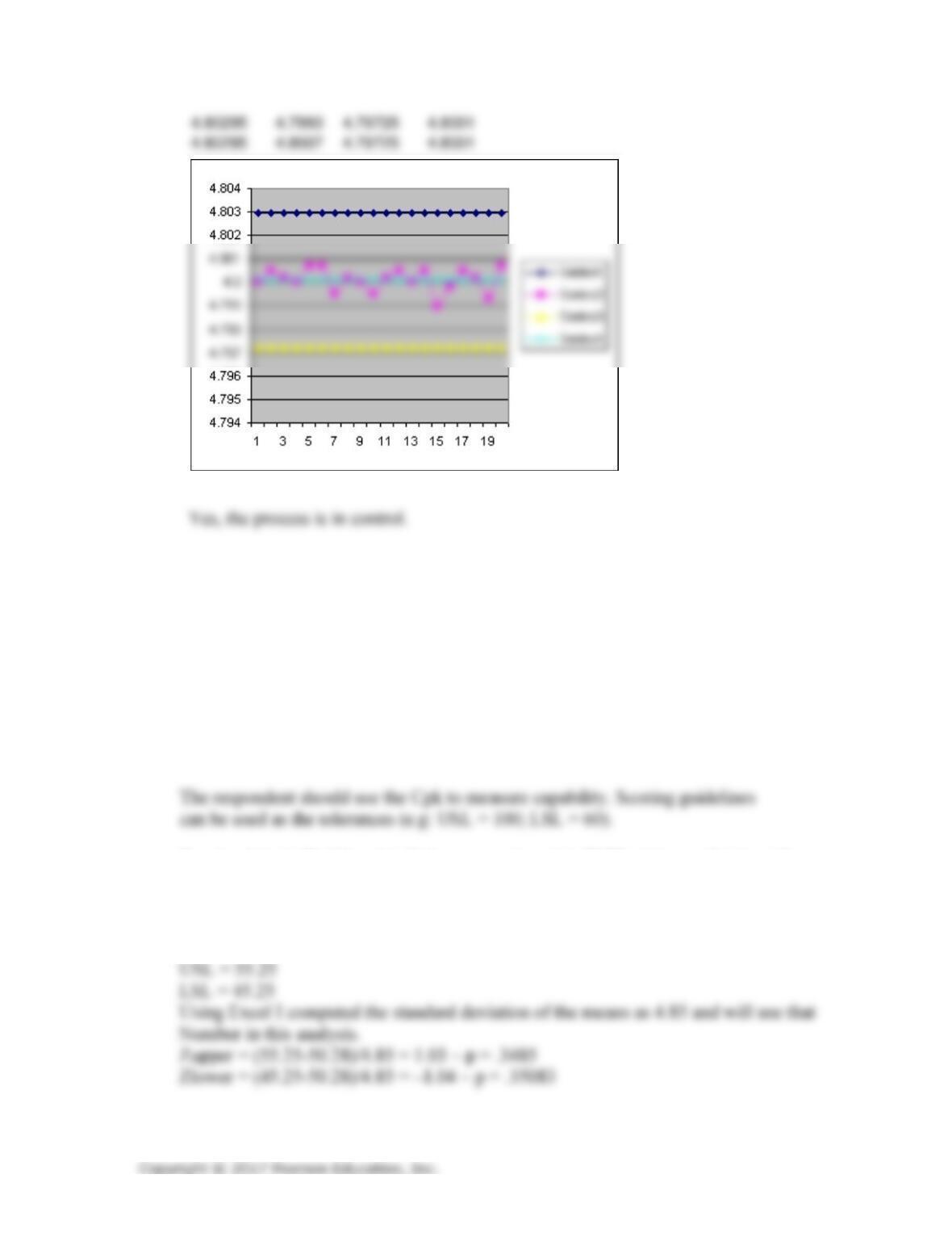
4.80295
4.799
4.79725
4.8001
Mean:
4.8001
R-bar:
0.0024
2
4.7995
4.8007
4.8005
0.0012
4.8005
4
4.7993
4.8
4.801
0.0017
4.8
6
4.801
4.8007
4.8
0.001
4.8007
8
4.8
4.8002
4.8002
0.0002
4.8002
9
4.8012
4.8
4.7998
0.0014
4.8
10
4.7988
4.7995
4.8002
0.0014
4.7995
11
4.8005
4.7998
4.8002
0.0007
4.8002
12
4.8005
4.7995
4.8012
0.0017
4.8005
14
4.8
4.8005
4.801
0.001
4.8005
16
4.7998
4.8007
4.7983
0.0024
4.7998
18
4.8
4.8002
4.8002
0.0002
4.8002
19
4.7993
4.7986
4.7995
0.0009
4.7993
20
4.8007
4.8017
4.7998
0.0019
4.8007
4.8029
4.8
4.79725
4.8001
4.8029
4.8005
4.79725
4.8001
4.8029
4.8
4.79725
4.8001
4.8029
4.8007
4.79725
4.8001
4.8029
4.8007
4.79725
4.8001
4.8029
4.7995
4.79725
4.8001
4.8029
4.8002
4.79725
4.8001
4.8029
4.7995
4.79725
4.8001
4.8029
4.8005
4.79725
4.8001
4.8029
4.8005
4.79725
4.8001
4.80295
4.7998
4.79725
4.8001
4.80295
4.8002
4.79725
4.8001
Page 29 of 30
24.
25.
26.
Design a control plan for exam scores for your quality management class.
Describe how you would gather data, what type of chart is needed, how to
gather data, how to interpret the data, how to identify causes, and remedial
action to be taken when out-of-control situations occur.
Answers will vary.
For the sampling plan from Problem 24, how would you measure process
capability?
For the data in Problem 16, if the process target is 50.25 with spec limits +/-5,
describe statistically the problems that would occur if you used your spec limits
on a control chart where n=5. Discuss type I and type II error.
Mean = 50.28
Page 30 of 30
About 70% of the sample means will fall within the specification limits. This means