Page 1 of 30
Chapter 11: Statistically Based Quality
Improvement for Variables
Chapter Outline
• Statistical Fundamentals
• Process Control Charts
• Some Control Chart Concepts for Variables
• Process Capability for Variables
• Other Statistical Techniques in Quality Management
Overview
The chapter begins on page 278 with a fascinating statement: … many people
view the topic of statistics with fear, loathing, and trembling. This chapter unravels the
seeming intricacies of statistical thought in a clear, process-oriented manner.
The text presents a series of tools. Each tool is presented in a situation-based
premise that illustrates not only the mechanics of the tool, but its use. The intent of the
chapter is to present tools that are useable.
Discussion Questions
1. Discuss the concept of control. Is control helpful? Isn’t being controlling a
negative?
Controlling is one of the managerial functions, like planning, organizing, staffing and
directing. It is an important function because it helps to check for errors and take
Page 2 of 30
Characteristics of control:
• Control is a continuous process.
2. The concept of statistical thinking is an important theme in this chapter. What
are some examples of statistical thinking?
On page 279, the author defines statistical thinking as being based on three concepts:
• All work occurs in a system of interconnected processes.
• All processes have variation; the amount of variation tends to be underestimated.
3. Sometimes you do well on exams. Sometimes you have bad days. What are the
assignable causes when you do poorly?
4. What is the relationship between statistical quality improvement and Deming’s 14
points?
The relationship is subtle, but present. Deming is instrumental to the philosophy of
continuing improvement. He talks about improved planning and stresses an environment
5. What are some applications of process charts in services? Could demerits (points
off for mistakes) be charted? How?
Process charts, as defined in the chapter, are tools for measuring quantifiable data. A
process chart could be used to measure a quantifiable property of a service environment.
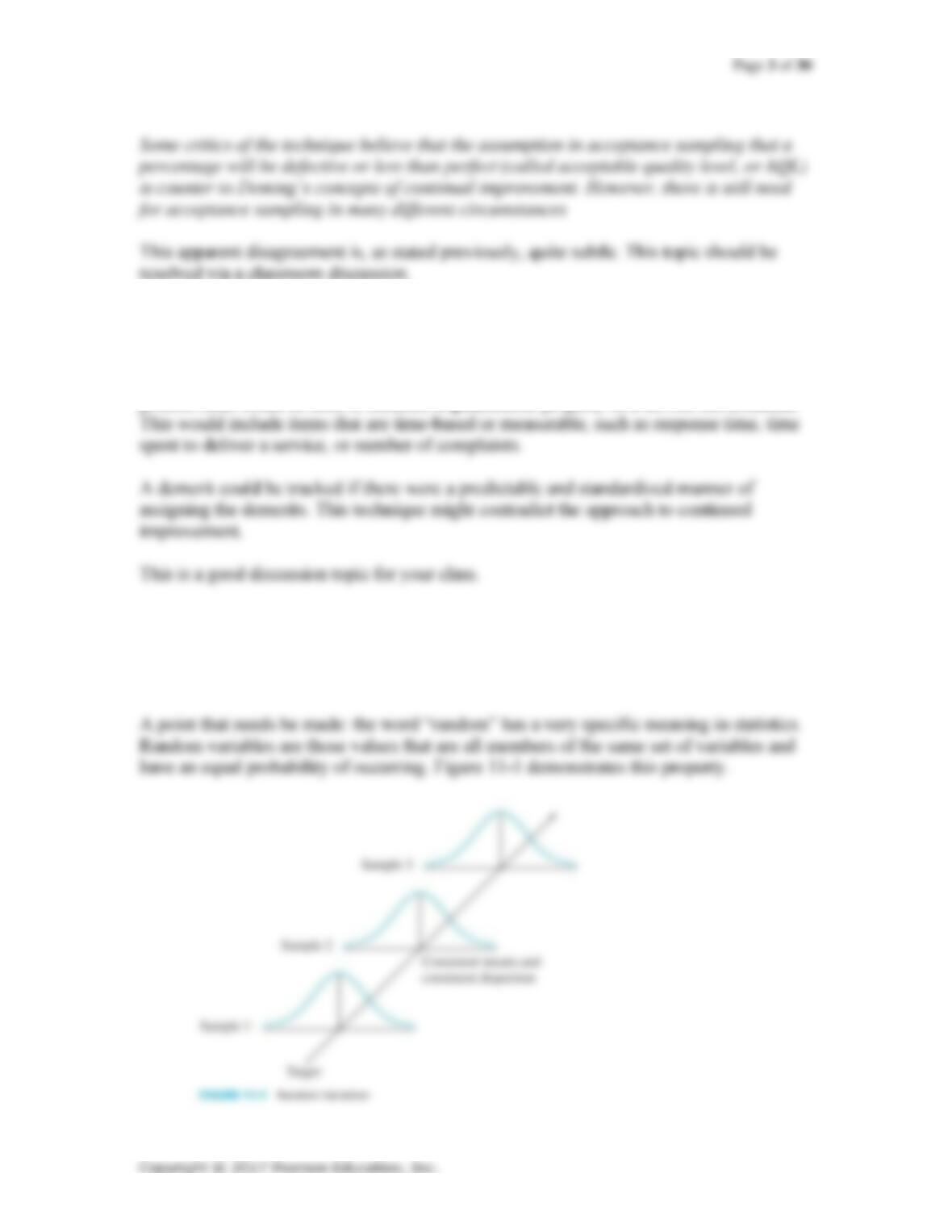
6. What is random variation? Is it always uncontrollable?
Random variation is that variation in a process that can be measured and analyzed. If it is
controlled, then by definition it is not random.
7. When would you choose an np chart over a p chart? An X chart over an x ¯
chart? An s chart over an R chart?
Charts are tools for portraying statistical information in an easy-to-comprehend manner.
A p chart presents the proportion of defective parts whereas an np chart presents the
number of non-conforming items. A p chart could be used to compare different items to
observe the difference in the processes.
8. Design a control chart to monitor the gas mileage in your car. Collect the data
over time. What did you find?
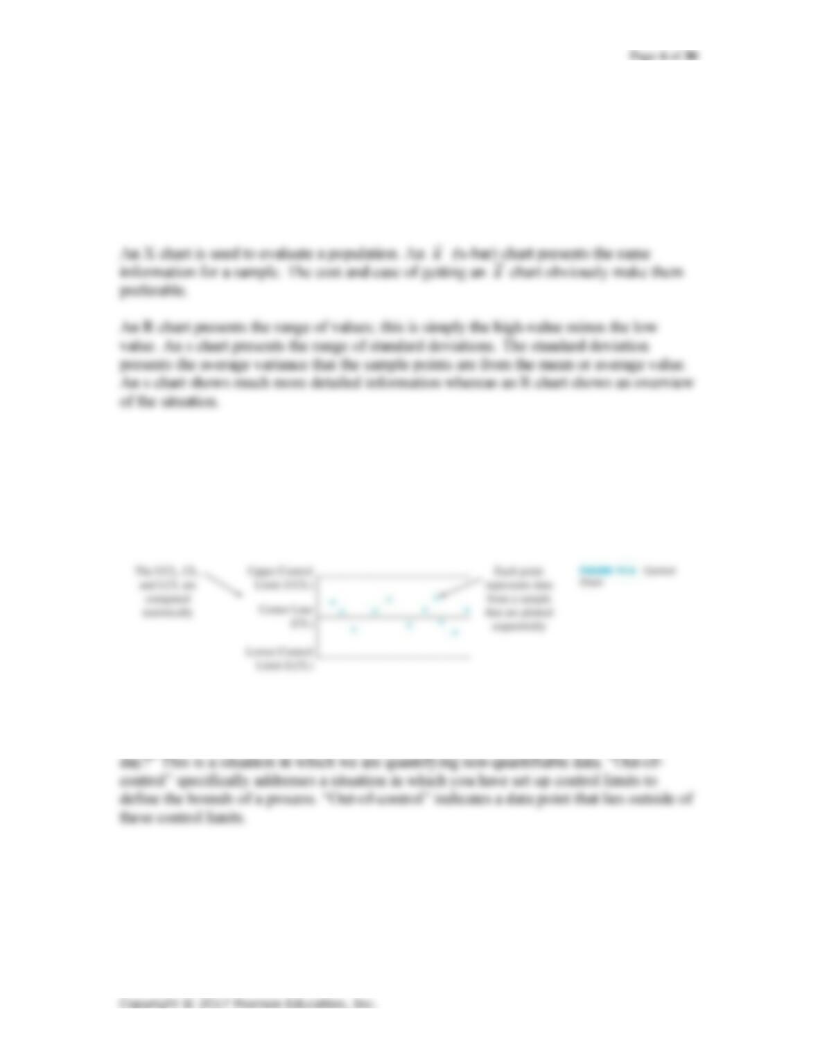
Figure 11-4 presents a simplified control chart. This will display the gas mileage over the
specified period of time. This might be a factor in a term paper.
9. What does “out-of-control” mean? Is it the same as a “bad hair day?”
How often do you have a “bad hair day?” How do you document or evaluate a “bad hair
10. Design a control chart to monitor the amounts of the most recently charged 50
debits from your debit card. What did you find?
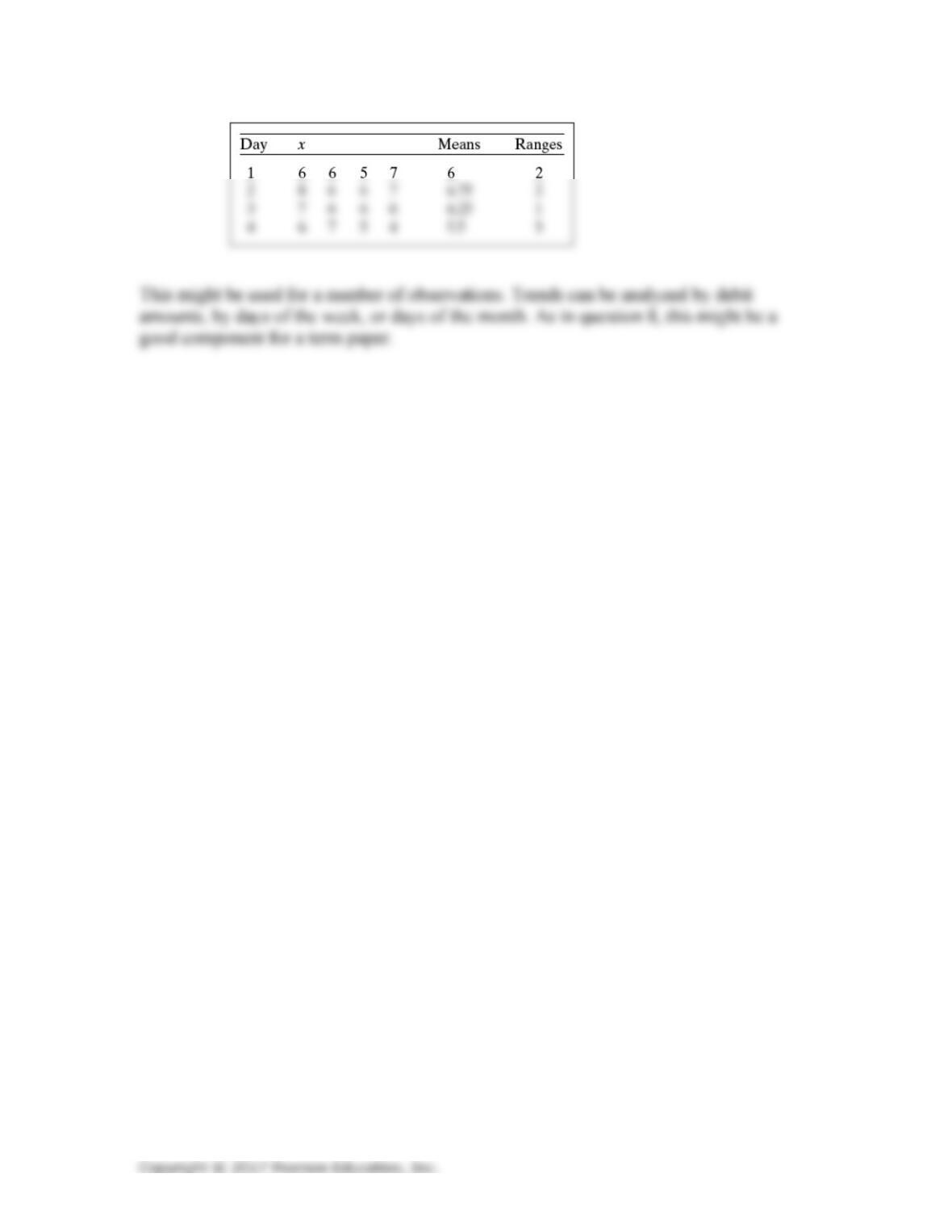
A debit is a highly quantifiable and measurable quantity. This data is ideal for statistical
analysis. A simple x ¯ chart might look like this:
Page 5 of 30
Case 11-1: Ore-Ida Fries
Take the data provided and use control charts to determine whether the
measurements are consistent. Report your results to management.
To develop this chart, do the following:
1. Load the data to Excel.
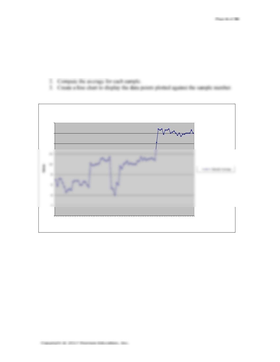
The results show a definite trend in the values.
0
14
16
18
1 4 7 10 13 16 19 22 25 28 31 34 37 40 43 46 49 52 55 58 61 64 67 70 73 76 79
Sample Number
Sample Averages for Ore-Ida UPC Code

Page 7 of 30
Suggested Answers to End of Chapter Problems
1.
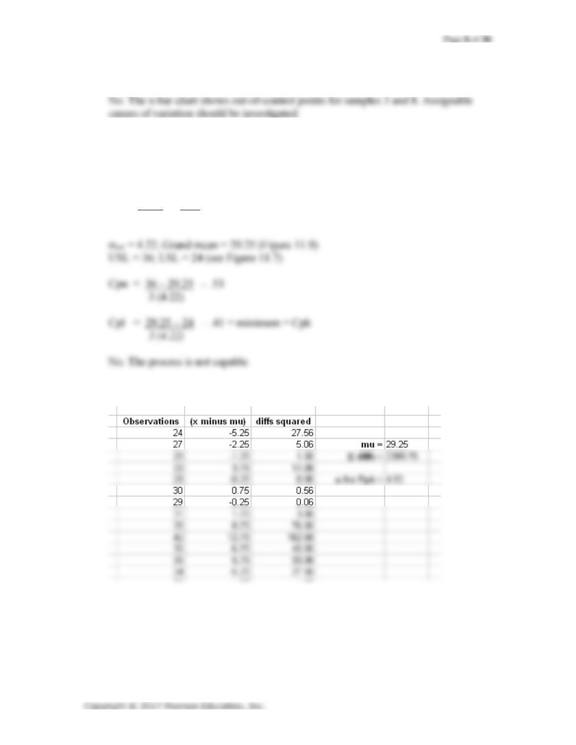
Return to the chart in Figure 11-8. Is this process stable?
2.
3.
Return to the data in Figure 11-8. Is this process capable? Compute both Cpk and Ppk.
Hint: Use the calculation work sheet to compute the population standard
deviation and for Ppk, treat each observation as a population value.
est. = R-bar = 8.68 (see Figure 11.9)
d2 2.059 (From Control Limits Factor Table)
For Ppk, standard deviation is 4.92 (see partial Excel printout below),
Ppu = .457 Ppl = .356 Ppk = .356 Process is not in control.
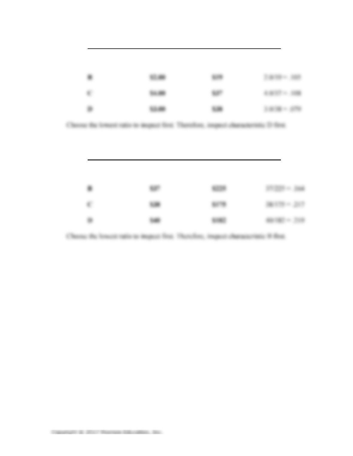
For the following product characteristics, choose where to inspect first:
Page 9 of 30
4.
Characteristic Cost of Inspection Cost of Failure Ratio
A $2.50 $20 2.5/20 = .125
For the following product characteristics, chose where to inspect first:
Characteristic Cost of Inspection Cost of Failure Ratio
A $35 $200 35/200 = .175
5.
6.
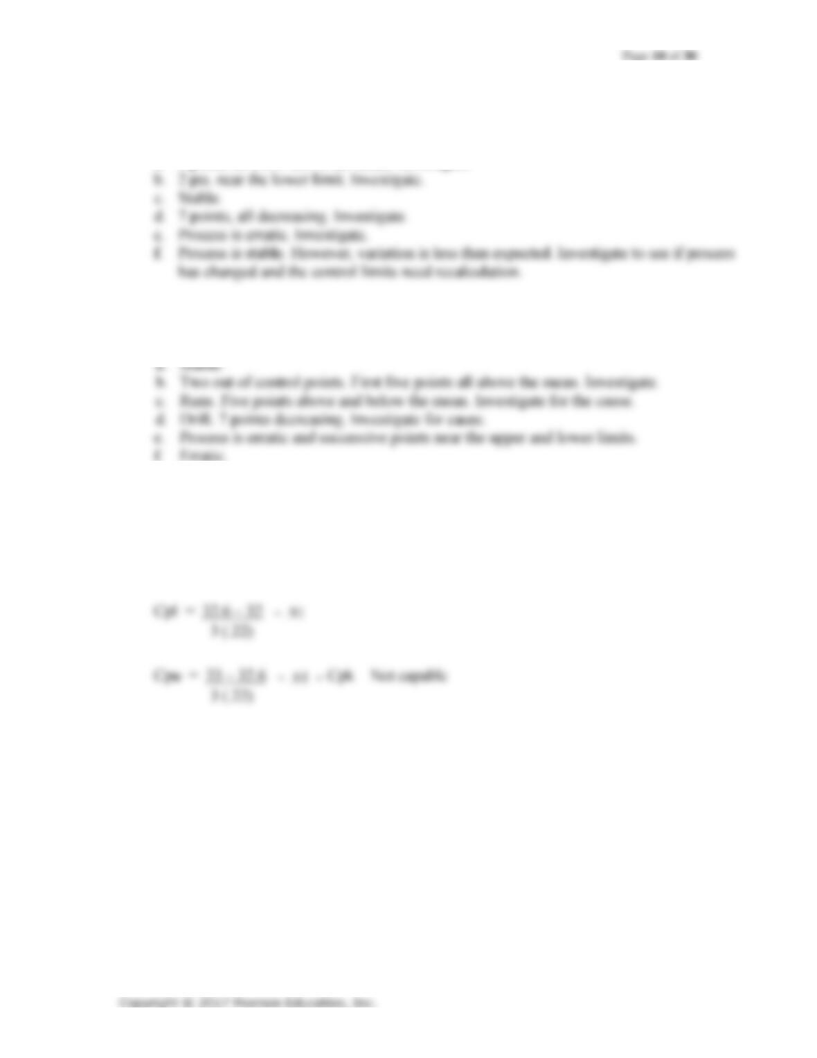
Interpret the charts in the text to determine if the processes are stable.
Answer:
a. 5 points in a row above the mean. Investigate.
Interpret the charts in the text to determine if the processes are stable.
Answer:
f. Erratic.
7.
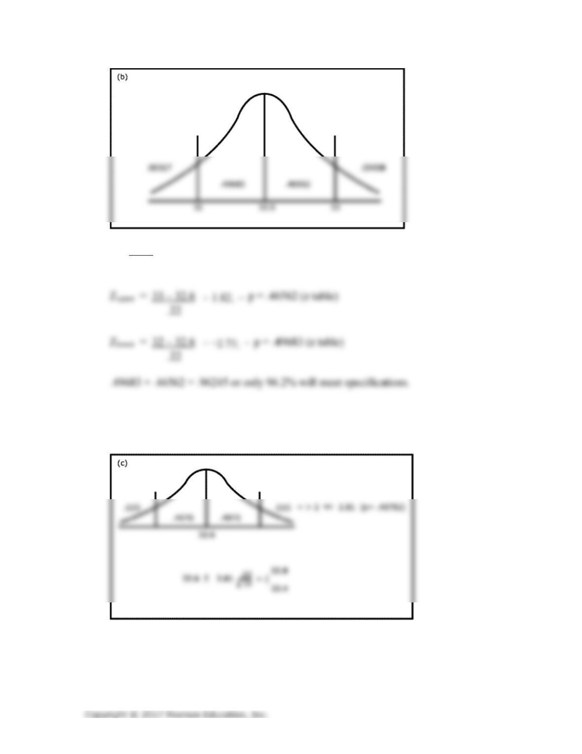
Tolerances for a new assembly call for weights between 32 and 33 pounds. The assembly
is made using a process that has a mean of 32.6 pounds with a population standard
deviation of .22 pounds. The process population is normally distributed.
a. Is the process capable?
b. If not, what proportion will meet tolerances?
Page 11 of 30
Z = x – m
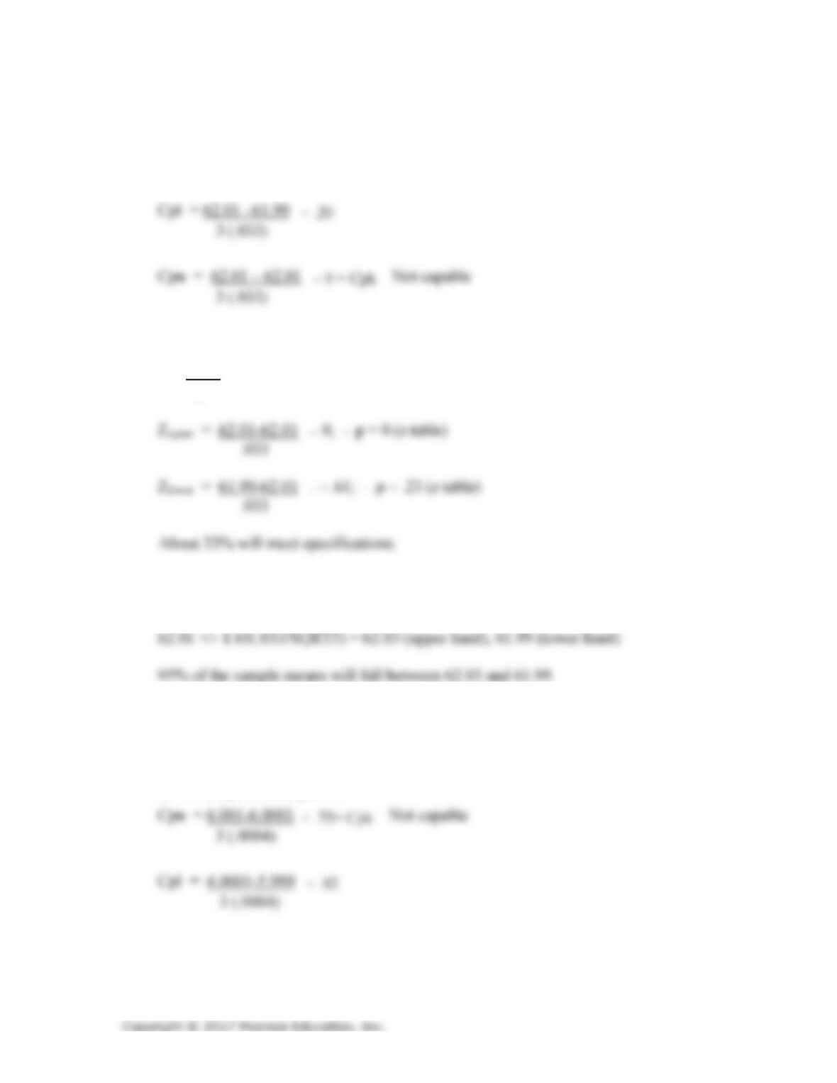
c. Within what values will 99.5% of sample means of this process fall if the sample size
is constant at 10 and the process is stable?
99.5% of sample means will fall between 32.4 and 32.8.
Page 12 of 30
8.
9.
Specifications for a part are 62” +/- .01”. The part is constructed from a process
with a mean of 62.01” and a population standard deviation of .033”. The process
is normally distributed.
a. Is the process capable?
b. What proportion will meet specifications?
Z = x – m
c. Within what values will 95% of sample means of the process fall if the sample size
is constant at 5 and the process is stable?
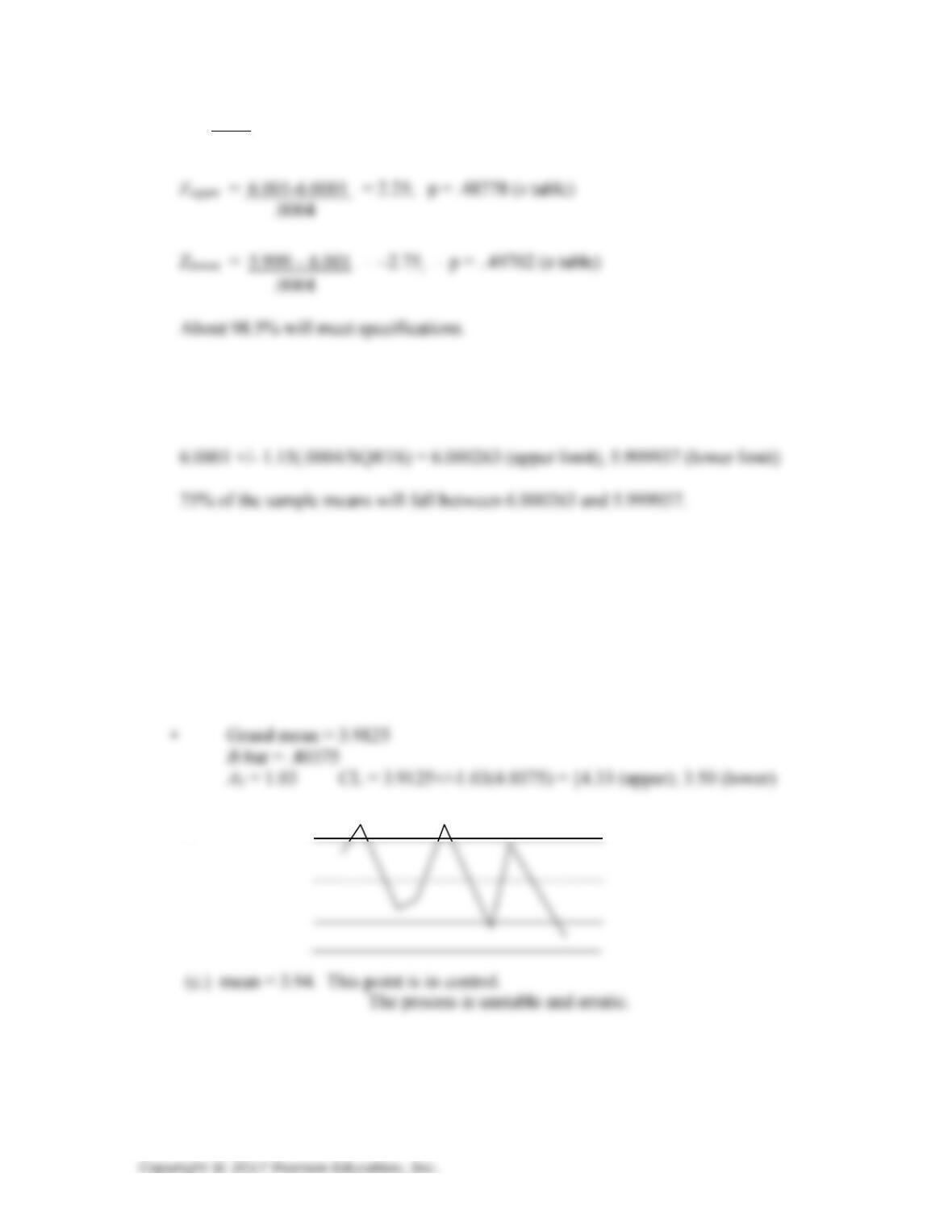
Tolerances for a bicycle derailleur are 6 cm +/- .001 cm. The current process
produces derailleurs with a mean of 6.0001 with a population standard deviation
of .0004. The process population is normally distributed.
a. Is the process capable?
b. If not, what proportion will meet specifications?
Page 13 of 30
10.
Z = x – m
c. Within what values will 75% of sample means of this process fall if the sample
size is constant at 6 and the process is stable?
A services process is monitored using x-bar and R charts. Eight samples of
n = 10 observations have been gathered with the following results:
a. Using the data in the table, compute the centerline, the upper control limit, and
the lower control limits for the x-bar and R charts.
b. Is the process in control? Please interpret the charts.
c. If the next sample results in the following values (2.5, 5.5, 4.6, 3.2, 4.6, 3.2, 4.0,
4.0, 3.6, 4.2), will the process be in control?
(b
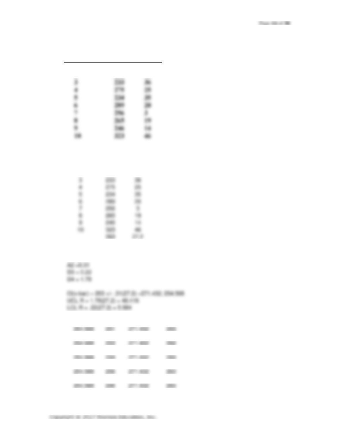
254.568
251
271.432
263
3
233
36
4
275
25
5
234
35
6
289
20
7
256
8
265
19
9
246
14
A2 =0.31
D3 = 0.22
D4 = 1.78
Cl(x-bar) = 263 +/- .31(27.2) =271.432; 254.568
UCL R = 1.78(27.2) = 48.416
LCL R = .22(27.2) = 5.984
11.
A production process for the JMF Semicon is monitored using x-bar and R charts.
10 samples of n=15 observations have been gathered with the following results:
Sample Mean Range
1 251 29
2 258 45
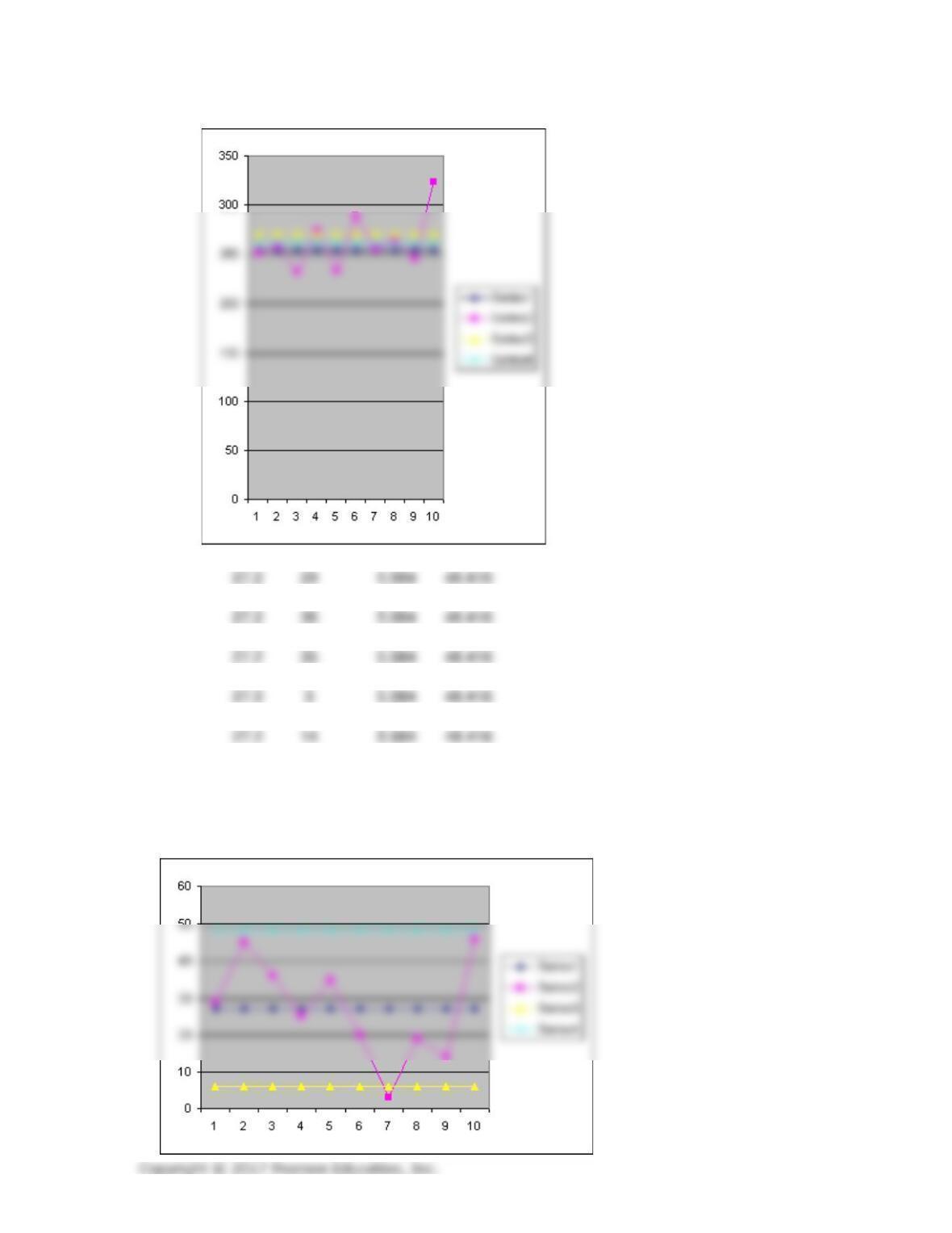
a. Develop a control chart and plot the means.
Sample
Mean
Range
1
251
29
2
258
45
263
27.2
Grand Mean = 263
R-bar = 27.2
n=10
X-bar Chart:
254.568
258
271.432
263
254.568
233
271.432
263
254.568
275
271.432
263
254.568
234
271.432
263
254.568
289
271.432
263
254.568
256
271.432
263
254.568
265
271.432
263
254.568
323
271.432
263
Page 15 of 30
27.2
29
5.984
48.416
27.2
14
5.984
48.416
27.2
45
5.984
48.416
27.2
36
5.984
48.416
27.2
25
5.984
48.416
27.2
35
5.984
48.416
27.2
20
5.984
48.416
27.2
5.984
48.416
27.2
19
5.984
48.416
27.2
46
5.984
48.416