Solved Problem 3
Master Scheduling
<Back
Week 0 1 2 3 4 5 6 7 8
Forecast 70 70 70 70
Customer Orders
Clear
Page 14
Chapter 11 – Problems 1-13 Note: This worksheet displays results only, you must copy the shaded
<Back area into the corresponding template to make additional calculations.
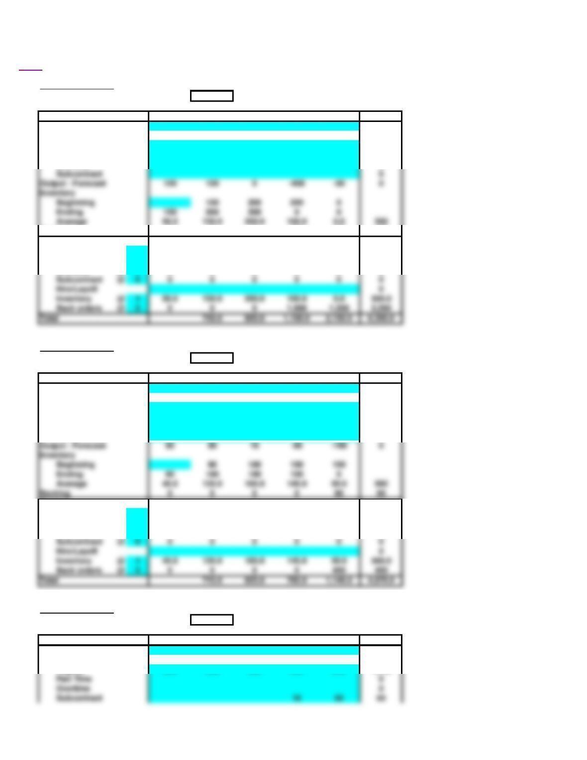
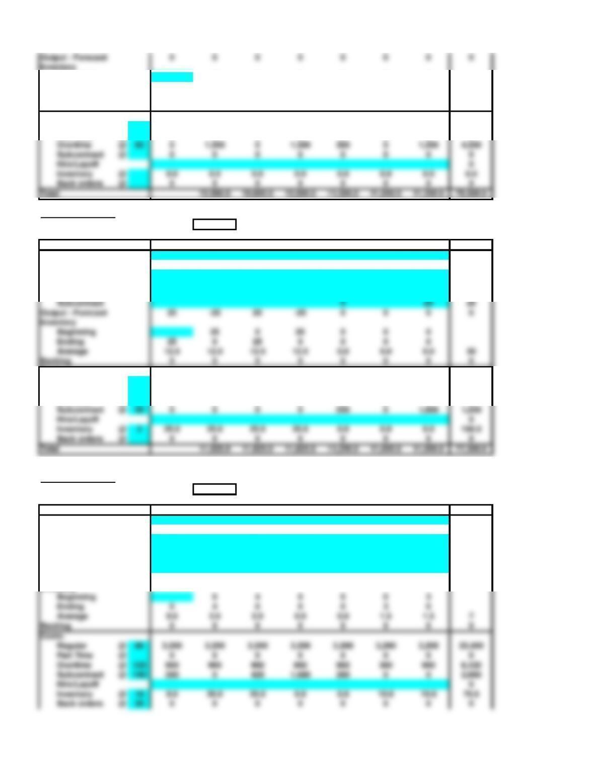
1. Aggregate Planning
Number of periods: 6
Period 1 2 3 4 5 Total
Forecast 200 200 300 400 500 1,800
Output
Regular 300 300 300 0450 1,800
Part Time 0
Overtime 0
Backlog 0 0 0 200 250 450
Costs:
Regular @ 2 600 600 600 0900 3,600
Part Time @ 0 0 0 0 0 0
Overtime @ 3 0 0 0 0 0 0
Subcontract @ 6 0 0 0 0 0 0
Hire/Layoff 0
Inventory @ 1 50.0 150.0 200.0 100.0 0.0 500.0
2a. Aggregate Planning
Number of periods: 6
Period 1 2 3 4 5 Total
Forecast 200 200 300 400 500 1,800
Output
Regular 290 290 290 290 290 1,740
Part Time 0
Overtime 20 20 20 60
Subcontract 0
Inventory
Costs:
Regular @ 2 580 580 580 580 580 3,480
Part Time @ 0 0 0 0 0 0
Overtime @ 3 0 0 60 60 60 180
Subcontract @ 6 0 0 0 0 0 0
Hire/Layoff 0
Inventory @ 1 45.0 135.0 185.0 145.0 50.0 560.0
2b. Aggregate Planning
Number of periods: 6
Period 1 2 3 4 5 Total
Forecast 200 200 300 400 500 1,800
Output
Regular 290 290 290 290 290 1,740
Part Time 0
Overtime 0
Subcontract 0
Inventory
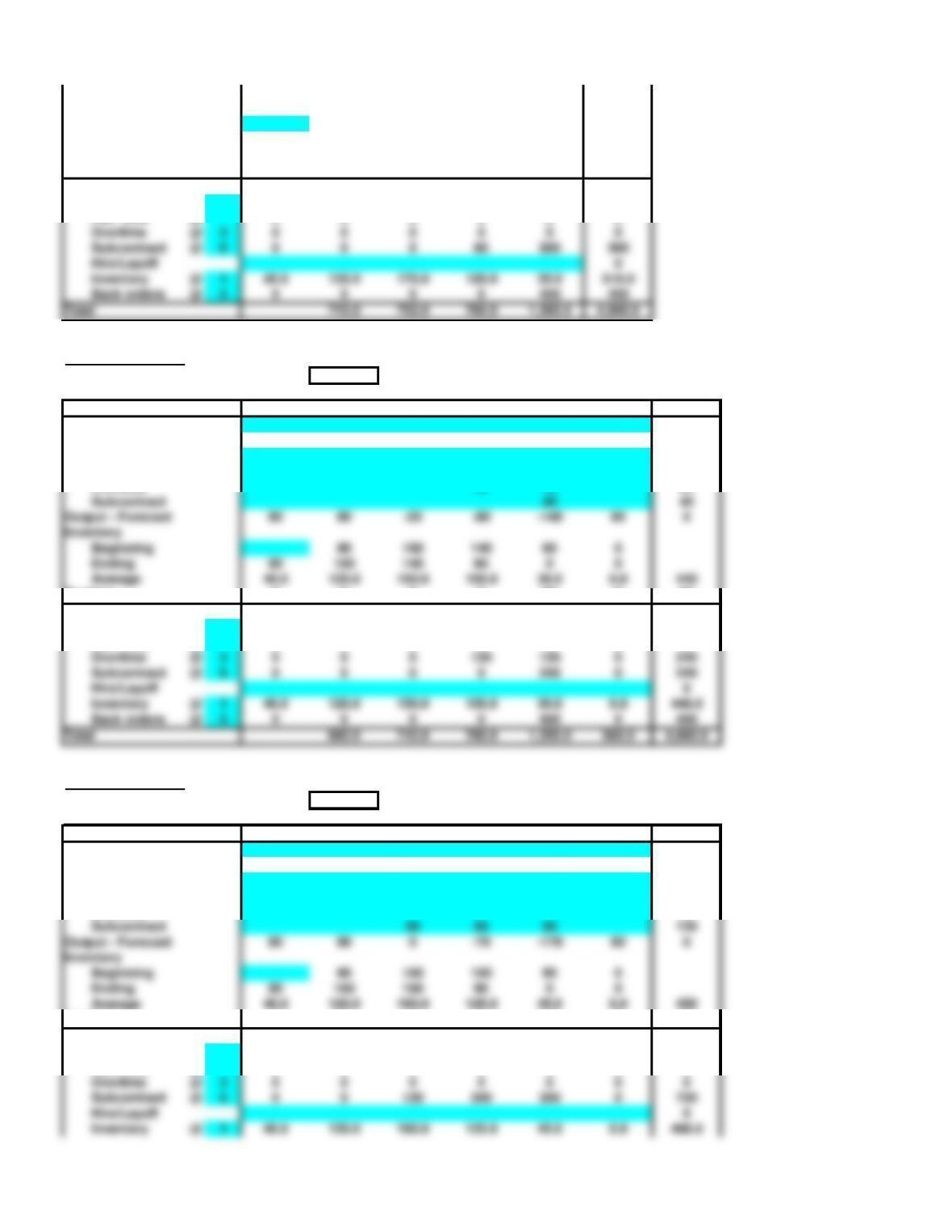
Output – Forecast 90 90 -10 -100 -160 0
Inventory
Beginning 90 180 170 70
Ending 90 180 170 70 0
Average 45.0 135.0 175.0 120.0 35.0 510
Backlog 0 0 0 0 90 90
Costs:
Regular @ 2 580 580 580 580 580 3,480
Part Time @ 0 0 0 0 0 0
3. Aggregate Planning
Number of periods: 6
Period 1 2 3 4 5 6 Total
Forecast 200 200 300 400 500 200 1,800
Output
Regular 280 280 280 280 280 280 1,680
Part Time 0
Overtime 40 40 80
Output – Forecast 80 80 -20 -80 -140 80 0
Inventory
Beginning 80 160 140 60 0
Ending 80 160 140 60 0 0
Average 40.0 120.0 150.0 100.0 30.0 0.0 440
Backlog 0 0 0 0 80 080
Costs:
Regular @ 2 560 560 560 560 560 560 3,360
Part Time @ 0 0 0 0 0 0 0
Overtime @ 3 0 0 0 120 120 0240
Subcontract @ 6 0 0 0 0 240 0240
Hire/Layoff 0
Inventory @ 1 40.0 120.0 150.0 100.0 30.0 0.0 440.0
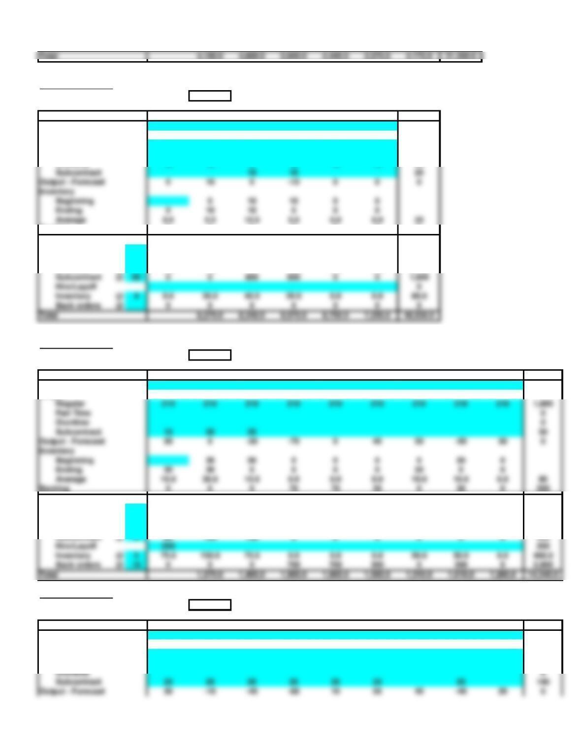
4. Aggregate Planning
Number of periods: 6
Period 1 2 3 4 5 6 Total
Forecast 200 200 300 400 500 200 1,800
Output
Regular 280 280 280 280 280 280 1,680
Part Time 0
Overtime 0
Output – Forecast 80 80 0 -70 -170 80 0
Inventory
Beginning 80 160 160 90 0
Ending 80 160 160 90 0 0
Average 40.0 120.0 160.0 125.0 45.0 0.0 490
Backlog 0 0 0 0 80 080
Costs:
Regular @ 2 560 560 560 560 560 560 3,360
Part Time @ 0 0 0 0 0 0 0
Subcontract @ 6 0 0 120 300 300 0720
Hire/Layoff 0
Inventory @ 1 40.0 120.0 160.0 125.0 45.0 0.0 490.0
Subcontract @ 6 0 0 0 60 300 360
Hire/Layoff 0
Inventory @ 1 45.0 135.0 175.0 120.0 35.0 510.0
Total 680.0 840.0 985.0 1,305.0 560.0 4,970.0
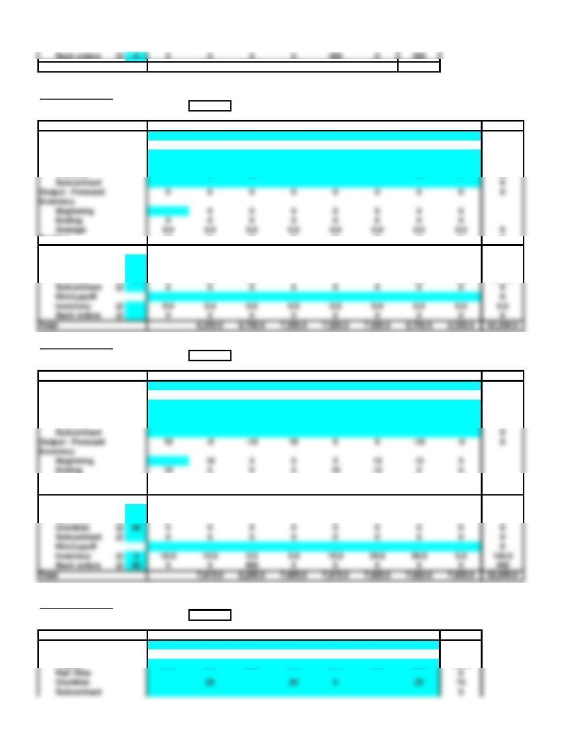
5a. Aggregate Planning
Number of periods: 8
Period 1 2 3 4 5 6 7 8 Total
Forecast 120 135 140 120 125 125 140 135 1,040
Output
Regular 120 130 130 120 125 125 130 130 1,010
Part Time 0
Overtime 5 10 10 530
Inventory
Backlog 0 0 0 0 0 0 0 0 0
Costs:
Regular @ 60 7,200 7,800 7,800 7,200 7,500 7,500 7,800 7,800 60,600
Part Time @ 0 0 0 0 0 0 0 0 0
Overtime @ 90 0450 900 0 0 0 900 450 2,700
Hire/Layoff 0
Total 8,250.0 8,700.0 7,200.0 7,500.0 7,500.0 8,700.0 8,250.0 63,300.0
5b. Aggregate Planning
Number of periods: 8
Period 1 2 3 4 5 6 7 8 Total
Forecast 120 135 140 120 125 125 140 135 1,040
Output
Regular 130 130 130 130 130 130 130 130 1,040
Part Time 0
Overtime 0
Inventory
Average 5.0 7.5 2.5 2.5 7.5 12.5 10.0 2.5 50
Backlog 0 0 5 0 0 0 0 0 5
Costs:
Regular @ 60 7,800 7,800 7,800 7,800 7,800 7,800 7,800 7,800 62,400
Part Time @ 0 0 0 0 0 0 0 0 0
Overtime @ 90 0 0 0 0 0 0 0 0 0
Hire/Layoff 0
Total 7,815.0 8,255.0 7,805.0 7,815.0 7,825.0 7,820.0 7,805.0 62,950.0
Aggregate Planning
Number of periods: 7
6a. Period 1 2 3 4 5 6 7 Total
Forecast 250 300 250 300 280 275 270 1,925
Output
Regular 250 275 250 275 275 275 250 1,850
Part Time 0
Beginning 0 0 0 0 0 0
Ending 0 0 0 0 0 0 0
Average 0.0 0.0 0.0 0.0 0.0 0.0 0.0 0
Backlog 0 0 0 0 0 0 0 0
Costs:
Regular @ 40 10,000 11,000 10,000 11,000 11,000 11,000 10,000 74,000
Part Time @ 0 0 0 0 0 0 0 0
Overtime @ 60 0 1,500 0 1,500 300 0 1,200 4,500
Subcontract @ 0 0 0 0 0 0 0 0
Hire/Layoff 0
Inventory @ 0.0 0.0 0.0 0.0 0.0 0.0 0.0 0.0
6b. Aggregate Planning
Number of periods: 7
Period 1 2 3 4 5 6 7 Total
Forecast 250 300 250 300 280 275 270 1,925
Output
Regular 275 275 275 275 275 275 250 1,900
Part Time 0
Overtime 0
Output – Forecast 25 -25 25 -25 0 0 0 0
Inventory
Backlog 0 0 0 0 0 0 0 0
Costs:
Regular @ 40 11,000 11,000 11,000 11,000 11,000 11,000 10,000 76,000
Part Time @ 0 0 0 0 0 0 0 0
Overtime @ 60 0 0 0 0 0 0 0 0
Hire/Layoff 0
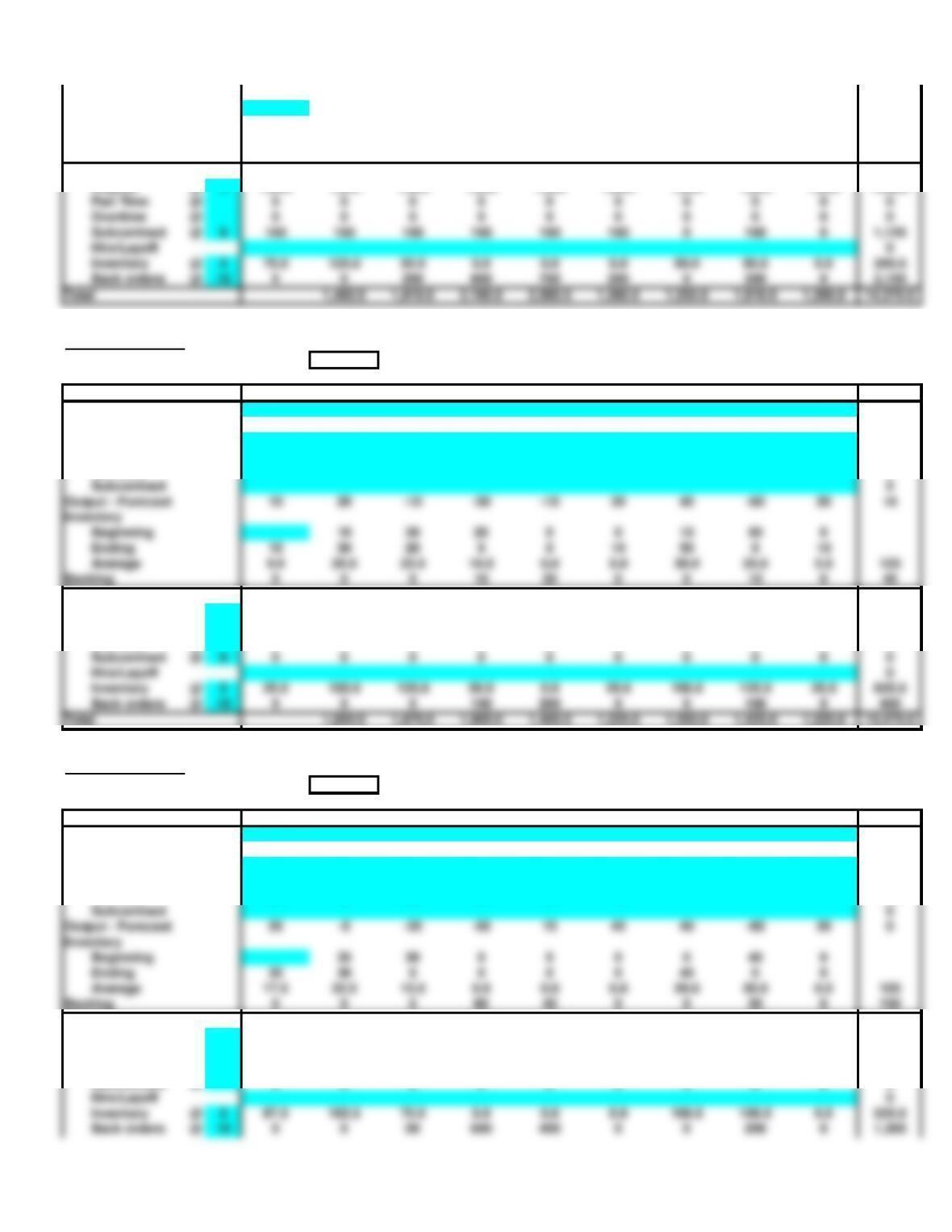
7a. Aggregate Planning
Number of periods: 7
Period 1 2 3 4 5 6 7 Total
Forecast 50 44 55 60 50 40 51 350
Output
Regular 40 40 40 40 40 40 40 280
Part Time 0
Overtime 8 8 8 8 8 3 8 51
Subcontract 2 3 12 219
Output – Forecast 0 4 -4 0 0 3 -3 0
Inventory
Beginning 0 4 0 0 0 3
Ending 0 4 0 0 0 3 0
Average 0.0 2.0 2.0 0.0 0.0 1.5 1.5 7
Backlog 0 0 0 0 0 0 0 0
Costs:
Regular @ 80 3,200 3,200 3,200 3,200 3,200 3,200 3,200 22,400
Part Time @ 0 0 0 0 0 0 0 0
Hire/Layoff 0
Output – Forecast 0 0 0 0 0 0 0 0
Inventory
9. Aggregate Planning
Number of periods: 6
Period 1 2 3 4 5 6 Total
Forecast 160 150 160 180 170 140 960
Output
Regular 150 150 150 150 160 130 890
Part Time 0
Overtime 10 10 010 10 10 50
Inventory
Backlog 0 0 0 0 0 0 0
Costs:
Regular @ 50 7,500 7,500 7,500 7,500 8,000 6,500 44,500
Part Time @ 0 0 0 0 0 0 0
Overtime @ 75 750 750 0750 750 750 3,750
Hire/Layoff 0
Total 8,270.0 8,340.0 9,070.0 8,750.0 7,250.0 49,930.0
10. Aggregate Planning
Number of periods: 9
Period 1 2 3 4 5 6 7 8 9 Total
Forecast 190 230 260 280 210 170 160 260 180 1,940
Output
Regular 210 210 210 210 210 210 210 210 210 1,890
Part Time 0
Inventory
Costs:
Regular @ 6 1,260 1,260 1,260 1,260 1,260 1,260 1,260 1,260 1,260 11,340
Part Time @ 0 0 0 0 0 0 0 0 0 0
Overtime @ 0 0 0 0 0 0 0 0 0 0
Hire/Layoff 200 200
Total 1,570.0 1,495.0 1,960.0 1,960.0 1,560.0 1,310.0 1,610.0 1,260.0 14,340.0
Aggregate Planning
Number of periods: 9
Period 1 2 3 4 5 6 7 8 9 Total
Forecast 190 230 260 280 210 170 160 260 180 1,940
Output
Regular 200 200 200 200 200 200 200 200 200 1,800
Part Time 0
Total 4,180.0 4,600.0 5,840.0 4,440.0 3,575.0 4,175.0 31,250.0
Inventory
Beginning 30 20 0 0 0 0 20 0
Ending 30 20 0 0 0 0 20 0 0
Average 15.0 25.0 10.0 0.0 0.0 0.0 10.0 10.0 0.0 70
Backlog 0 0 20 80 70 20 020 0210
Costs:
Regular @ 6 1,200 1,200 1,200 1,200 1,200 1,200 1,200 1,200 1,200 10,800
11. Aggregate Planning
Number of periods: 9
Period 1 2 3 4 5 6 7 8 9 Total
Forecast 190 230 260 280 210 170 160 260 180 1,940
Output
Regular 200 200 200 200 200 200 200 200 200 1,800
Part Time 50 50 50 150
Overtime 0
Inventory
Beginning 10 30 20 0 0 10 50 0
Ending 10 30 20 0 0 10 50 010
Costs:
Regular @ 6 1,200 1,200 1,200 1,200 1,200 1,200 1,200 1,200 1,200 10,800
Part Time @ 11 0550 550 550 0 0 0 0 0 1,650
Overtime @ 0 0 0 0 0 0 0 0 0 0
Subcontract @ 8 0 0 0 0 0 0 0 0 0 0
Hire/Layoff 0
12. Aggregate Planning
Number of periods: 9
Period 1 2 3 4 5 6 7 8 9 Total
Forecast 190 230 260 280 210 170 160 260 180 1,940
Output
Regular 200 200 200 200 200 200 200 200 200 1,800
Part Time 0
Overtime 25 25 25 25 25 15 140
Inventory
Beginning 35 30 0 0 0 0 40 0
Ending 35 30 0 0 0 0 40 0 0
Average 17.5 32.5 15.0 0.0 0.0 0.0 20.0 20.0 0.0 105
Costs:
Regular @ 6 1,200 1,200 1,200 1,200 1,200 1,200 1,200 1,200 1,200 10,800
Part Time @ 0 0 0 0 0 0 0 0 0 0
Overtime @ 9 225 225 225 225 225 135 0 0 0 1,260
Subcontract @ 0 0 0 0 0 0 0 0 0 0
Hire/Layoff 0
Inventory @ 5 87.5 162.5 75.0 0.0 0.0 0.0 100.0 100.0 0.0 525.0
Part Time @ 0 0 0 0 0 0 0 0 0 0
Overtime @ 0 0 0 0 0 0 0 0 0 0
Subcontract @ 8 160 160 160 160 160 160 0160 0 1,120
Hire/Layoff 0
Inventory @ 5 75.0 125.0 50.0 0.0 0.0 0.0 50.0 50.0 0.0 350.0
Total 1,587.5 1,550.0 2,025.0 1,875.0 1,335.0 1,300.0 1,500.0 1,200.0 13,885.0
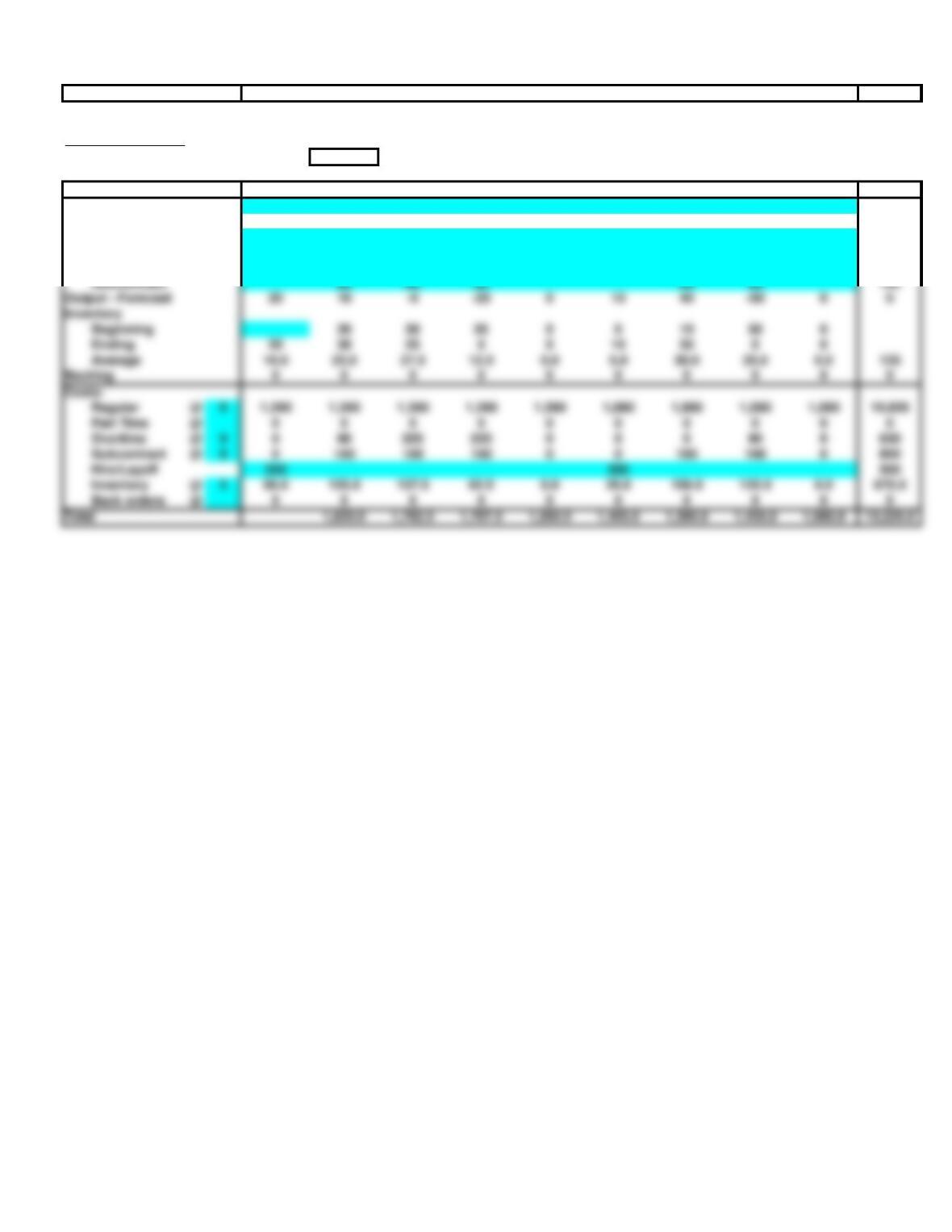
13. Aggregate Planning
Number of periods: 9
Period 1 2 3 4 5 6 7 8 9 Total
Forecast 190 230 260 280 210 170 160 260 180 1,940
Output
Regular 210 210 210 210 210 180 180 180 180 1,770
Part Time 0
Overtime 10 25 25 10 70
Inventory
Costs:
Part Time @ 0 0 0 0 0 0 0 0 0 0
Hire/Layoff 200 300 500
Total 1,635.0 1,782.5 1,707.5 1,260.0 1,405.0 1,390.0 1,455.0 1,080.0 13,225.0
Chapter 11 – Problems 14-19 Note: This worksheet displays results only, you must copy the shaded
<Back area into the corresponding template to make additional calculations.
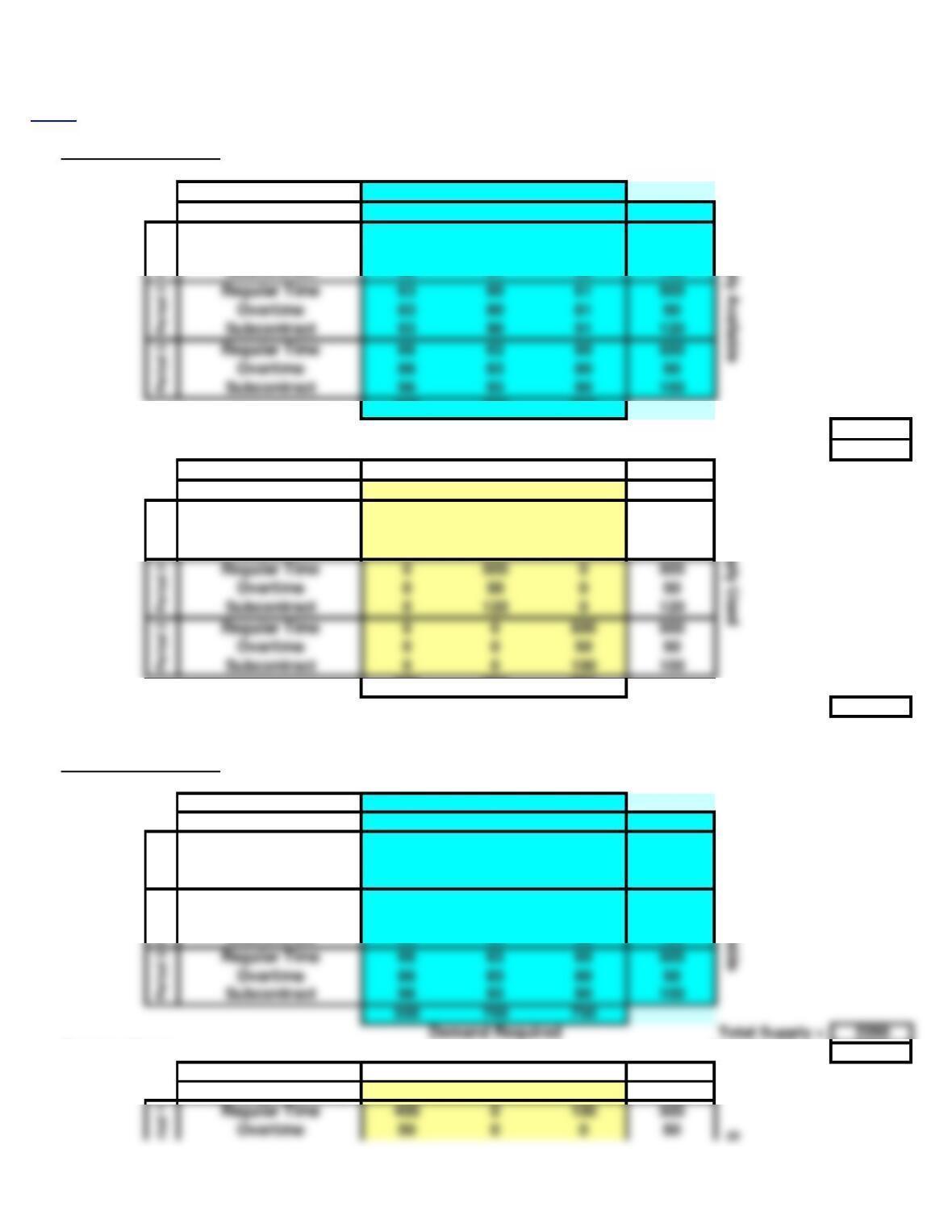
14. Transportation Model
Input Matrix: Demand for: Period 1 Period 2 Period 3
Beginning Inventory 0 1 2 100
Regular Time 60 61 62 500
Overtime 80 81 82 50
Subcontract 90 91 92 120
550 700 750
Demand Required Total Supply = 2090
Solution Matrix: Total Demand = 2000
Demand for: Period 1 Period 2 Period 3 0
Beginning Inventory 100 0 0 100
Regular Time 400 0100 500
Overtime 50 0 0 50
Subcontract 0 30 030
Regular Time 0 500 0500
Regular Time 0 0 500 500
Period 2
Period 3
550 700 750
Demand Met Total Cost = 124730
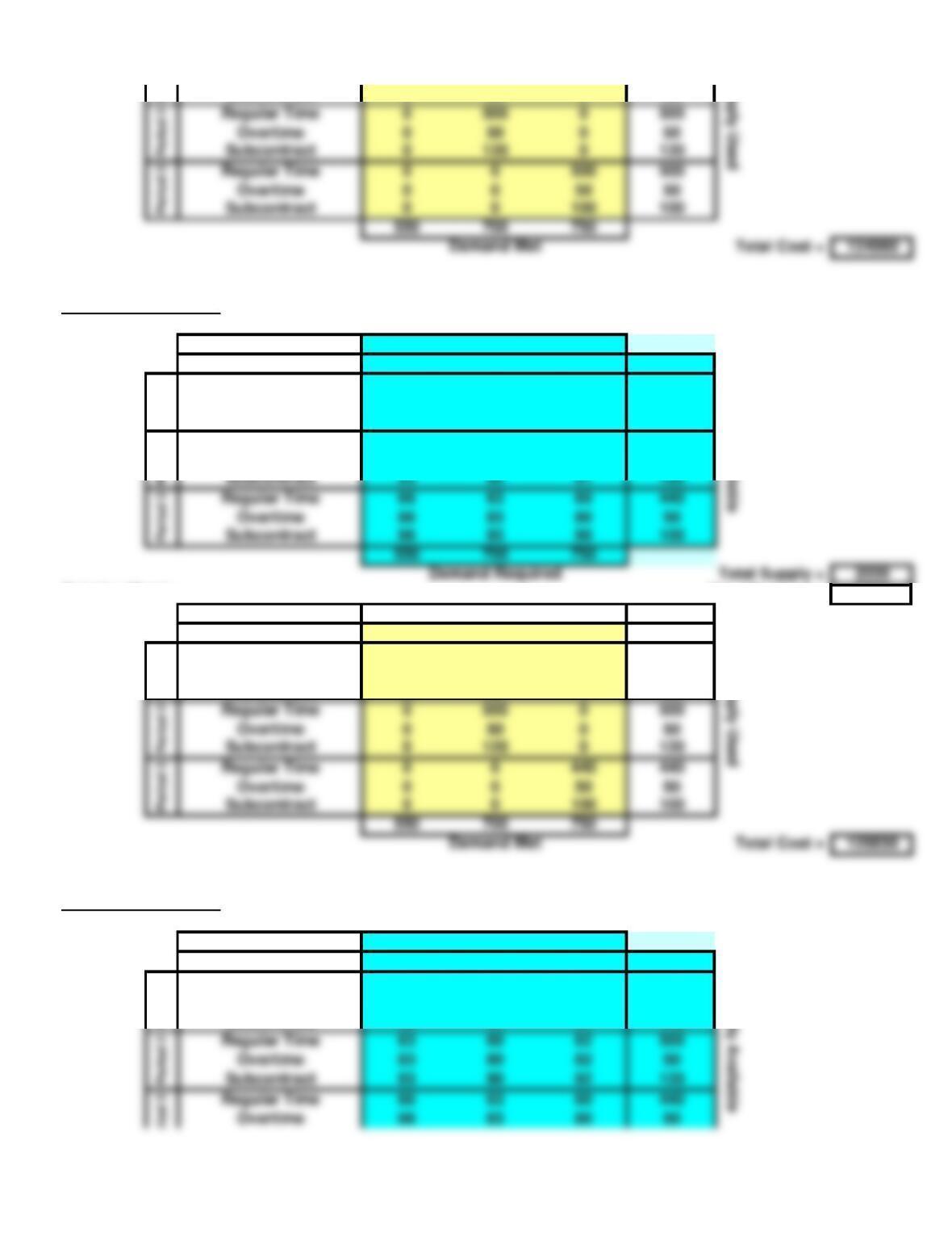
15. Transportation Model
Input Matrix: Demand for: Period 1 Period 2 Period 3
Beginning Inventory 0 2 4 100
Regular Time 60 62 64 500
Overtime 80 82 84 50
Subcontract 90 92 94 120
Regular Time 63 60 62 500
Overtime 83 80 82 50
Subcontract 93 90 92 120
Regular Time 66 63 60 500
Overtime 86 83 80 50
Subcontract 96 93 90 100
550 700 750
Demand Required Total Supply = 2090
Period 2
Period 3
Solution Matrix: Total Demand = 2000
Demand for: Period 1 Period 2 Period 3 0
Beginning Inventory 100 0 0 100
Regular Time 400 0100 500
Overtime 50 0 0 50
Supply Used
Period 1
Supply Available
Supply Available
Period 1
Regular Time 63 60 61 500
Overtime 83 80 81 50
Subcontract 93 90 91 120
Regular Time 66 63 60 500
Overtime 86 83 80 50
Subcontract 96 93 90 100
Period 2
Period 3
Period 1
Subcontract 0 30 030
16. Transportation Model
Input Matrix: Demand for: Period 1 Period 2 Period 3
Beginning Inventory 0 1 2 100
Regular Time 60 61 62 500
Overtime 80 81 82 50
Subcontract 90 91 92 120
Regular Time 63 60 61 500
Overtime 83 80 81 50
Subcontract 93 90 91 120
Regular Time 66 63 60 440
Overtime 86 83 80 50
Subcontract 96 93 90 100
Period 2
Period 3
Solution Matrix: Total Demand = 2000
Demand for: Period 1 Period 2 Period 3 0
Beginning Inventory 100 0 0 100
Regular Time 340 0160 500
Overtime 50 0 0 50
Subcontract 60 30 090
Regular Time 0 500 0500
Regular Time 0 0 440 440
Period 2
Period 3
17. Transportation Model
Input Matrix: Demand for: Period 1 Period 2 Period 3
Beginning Inventory 0 2 4 100
Regular Time 60 62 64 500
Overtime 80 82 84 50
Subcontract 90 92 94 120
Regular Time 63 60 62 500
Overtime 83 80 82 50
Regular Time 66 63 60 440
Overtime 86 83 80 50
Supply Available
Period 1
Supply Available
Period 1
Supply Used
Period 1
Supply Used
Pe
Regular Time 0 0 500 500
Period 2
Period 3
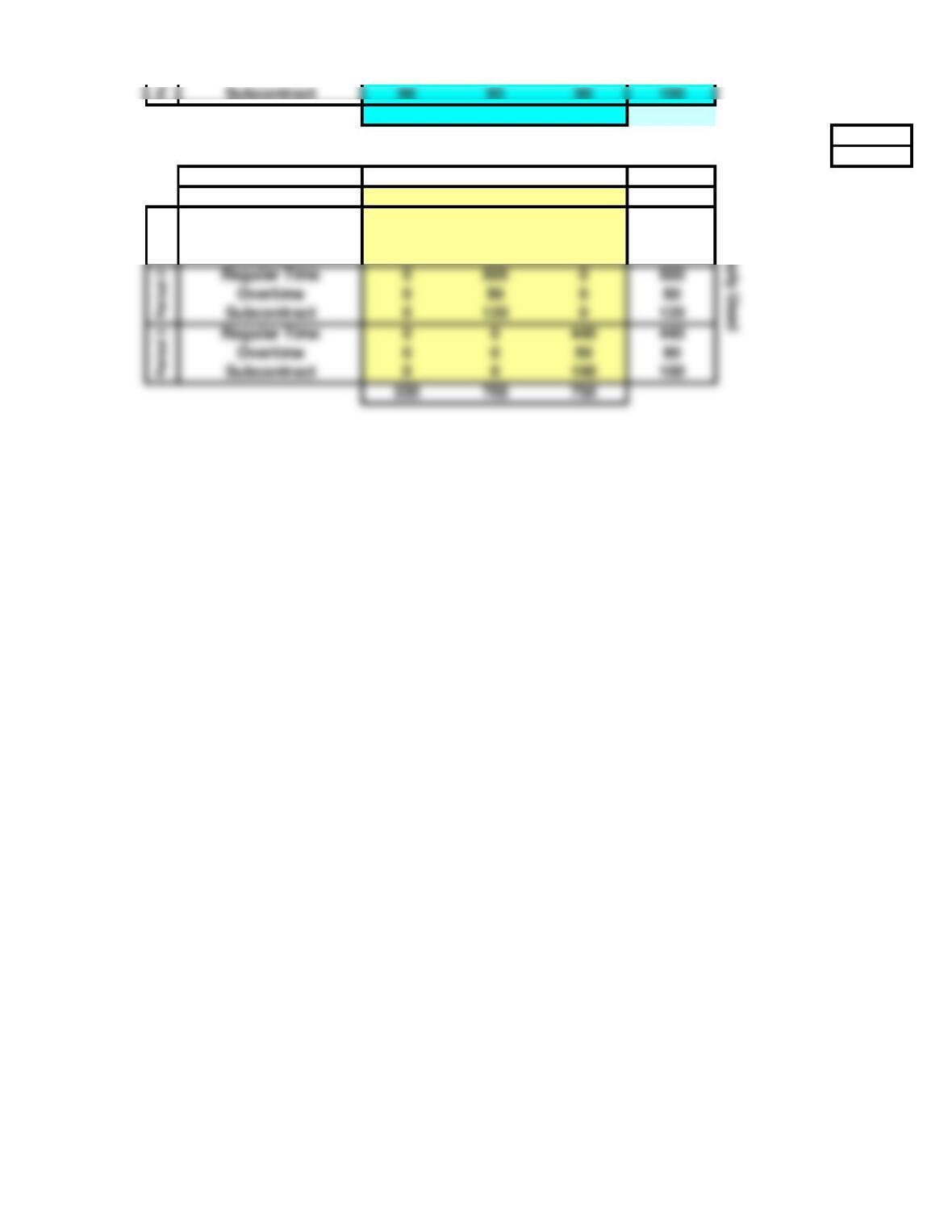
550 700 750
Demand Required Total Supply = 2030
Solution Matrix: Total Demand = 2000
Demand for: Period 1 Period 2 Period 3 0
Beginning Inventory 100 0 0 100
Regular Time 340 0160 500
Overtime 50 0 0 50
Subcontract 60 30 090
Regular Time 0 500 0500
Regular Time 0 0 440 440
Period 2
Pe
Supply Used
Period 1
Subcontract 96 93 90 100
Chapter 11 – Problems 20-23 Note: This worksheet displays results only, you must copy the shaded
<Back area into the corresponding template to make additional calculations.
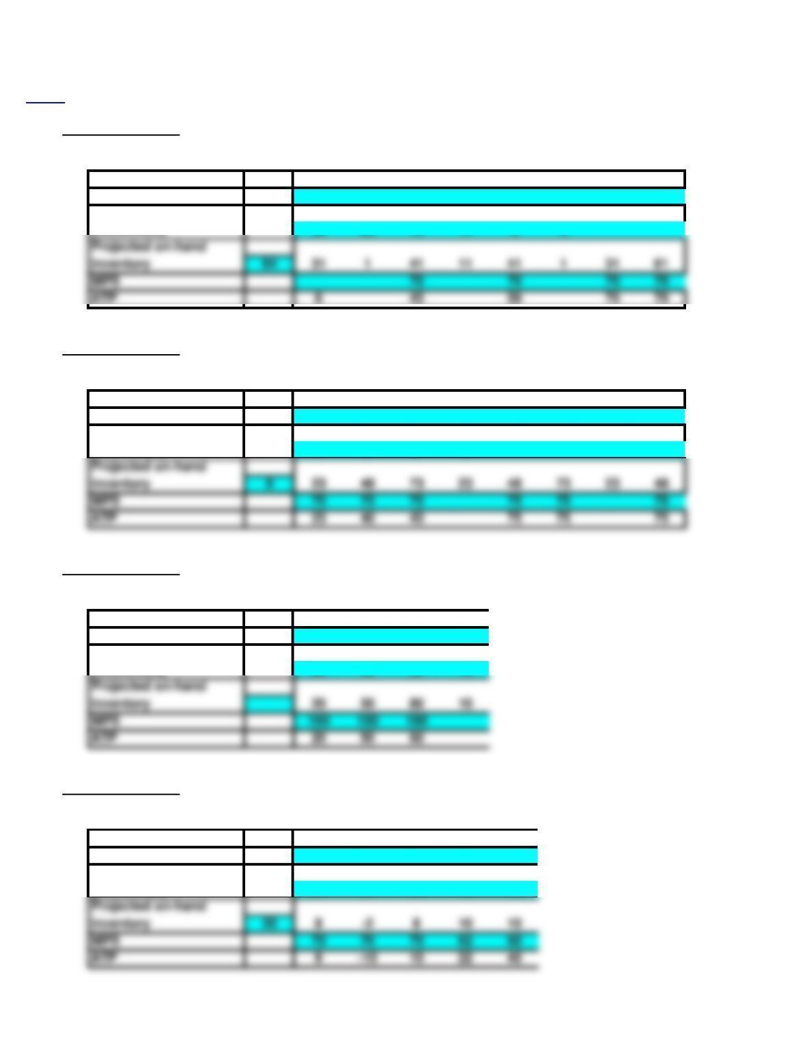
20. Master Scheduling
Week 0 1 2 3 4 5 6 7 8
Forecast 30 30 30 30 40 40 40 40
Customer Orders
(committed) 33 25 16 11 8 3
21. Master Scheduling
Week 0 1 2 3 4 5 6 7 8
Forecast 50 50 50 50 50 50 50 50
Customer Orders
(committed) 52 35 20 12
Projected on-hand
22. Master Scheduling
Week 0 1 2 3 4
Forecast 70 70 70 70
Customer Orders
(committed) 80 50 30 10
Projected on-hand
23. Master Scheduling
Week 0 1 2 3 4 5
Forecast 80 80 60 60 60
Customer Orders
(committed) 82 80 60 40 20
Projected on-hand