Chapter 11 – Aggregate Planning and Master Scheduling
11-13
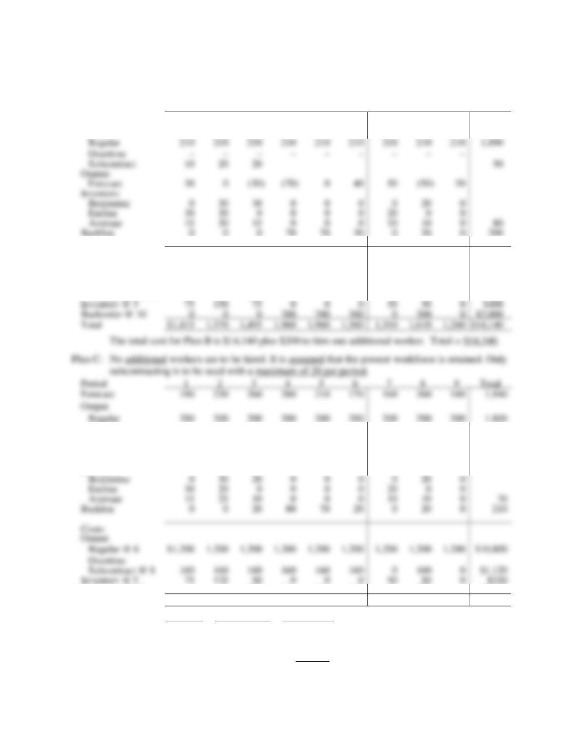
10. Plan B: Hire one worker and subcontract. Workforce = 20 + 1 = 21 workers.
Period
1
2
3
4
5
6
7
8
9
Total
Forecast
190
230
260
280
210
170
160
260
180
1,940
Output
Costs:
Output
Regular @ 6
$1,260
1,260
1,260
1,260
1,260
1,260
1,260
1,260
1,260
$11,340
Overtime
Subcontract @ 8
80
160
160
0
0
0
0
0
0
$400
Inventory @ 5
75
150
75
0
0
0
50
50
0
$400
Backorder @ 10
0
0
0
700
700
300
0
300
0
Total
$1,415
1,570
1,495
1,960
1,960
1,560
1,310
1,610
1,260
Forecast
190
230
260
280
210
170
160
260
180
Output
Regular
200
200
200
200
200
200
200
200
200
Overtime
–
–
–
–
–
–
–
–
–
Subcontract
20
20
20
20
20
20
0
20
0
140
Output-
Forecast
30
(10)
(40)
(60)
10
50
40
(40)
20
Inventory
Beginning
0
30
20
0
0
0
0
20
0
Ending
30
20
0
0
0
0
20
0
0
Average
15
25
10
0
0
0
10
10
0
Backlog
0
0
20
80
70
20
0
20
0
210
Costs:
Output
Regular @ 6
$1,200
1,200
1,200
1,200
1,200
1,200
1,200
1,200
1,200
$10,800
Overtime
Subcontract @ 8
160
160
160
160
160
160
0
160
0
$1,120
Inventory @ 5
75
125
50
0
0
0
50
50
0
Backorder @ 10
0
0
200
800
700
200
0
200
0
$2,100
Total
$1,435
1,485
1,610
2,160
2,060
1,560
1,250
1,610
1,200
$14,370
Plan
Total Cost
Rank
A
$14,290
3
B
14,370
2
C
14,370
1
The lowest cost is for Plan A = $14,290.
Regular
210
210
210
210
210
210
210
210
210
1,890
Overtime
–
–
–
–
–
–
–
–
–
Subcontract
10
20
20
Output-
Forecast
30
0
(30)
(70)
0
40
50
(50)
30
Inventory
Beginning
0
30
30
0
0
0
0
20
0
Ending
30
30
0
0
0
0
20
0
0
Average
15
30
15
0
0
0
10
10
0
Backlog
0
0
0
70
70
30
0
30
0
200
Chapter 11 – Aggregate Planning and Master Scheduling
11-14
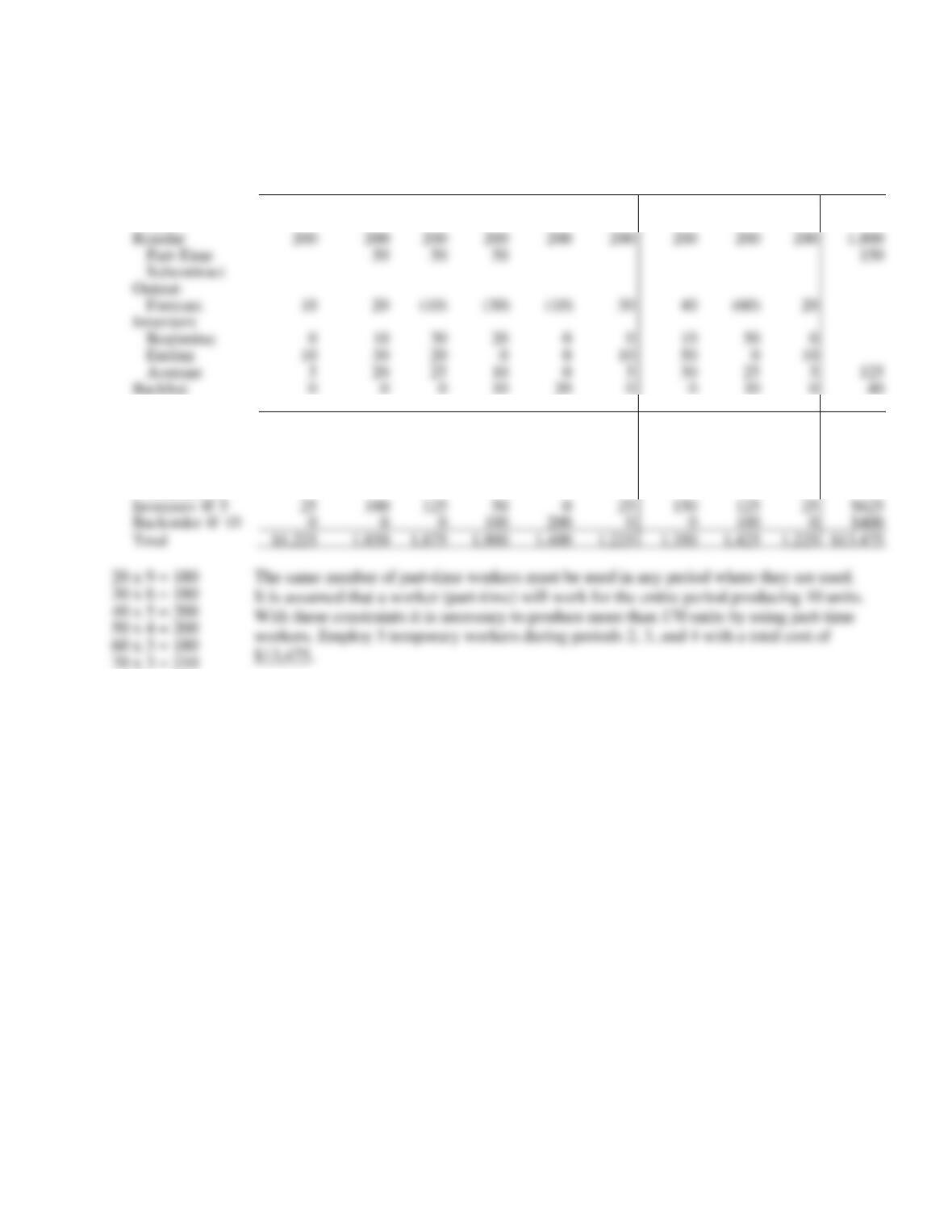
11. Assume that the $5 cost per unit for the temporary workers is in addition to $6 per unit for regular
time cost. Part-time workers are to be hired to produce at least 170 units.
Period
1
2
3
4
5
6
7
8
9
Total
Forecast
190
230
260
280
210
170
160
260
180
1,940
Output
Costs:
Output
Regular @ 6
$1,200
1,200
1,200
1,200
1,200
1,200
1,200
1,200
1,200
$10,800
Part-Time @ 11
550
550
550
$1,650
Subcontract
Backorder @ 10
100
200
100
Total
Regular
200
200
200
200
200
200
200
200
200
Part-Time
Subcontract
Output-
Inventory
Beginning
Ending
Average
Backlog
Chapter 11 – Aggregate Planning and Master Scheduling
11-15
12. Objective here is to minimize backlogs.
Period
1
2
3
4
5
6
7
8
9
Total
Forecast
190
230
260
280
210
170
160
260
180
2,570
Output
Regular
200
200
200
200
200
200
200
200
200
2,400
Overtime
25
25
25
25
25
15
170
Subcontract
0
0
0
0
0
0
0
0
0
Output-
Forecast
35
(5)
(35)
(55)
15
45
40
(60)
20
Inventory
Beginning
0
35
30
0
0
0
0
40
0
Ending
35
30
40
Average
17.5
15
0
0
0
20
20
0
Backlog
60
45
20
130
Output
Regular @ 6
$1,200
$10,800
Overtime @ 9
225
225
225
225
225
135
0
0
Subcontract
Inventory @ 5
87.5
75
0
0
0
100
100
0
$525
Backorder @ 10
50
Chapter 11 – Aggregate Planning and Master Scheduling
11-16
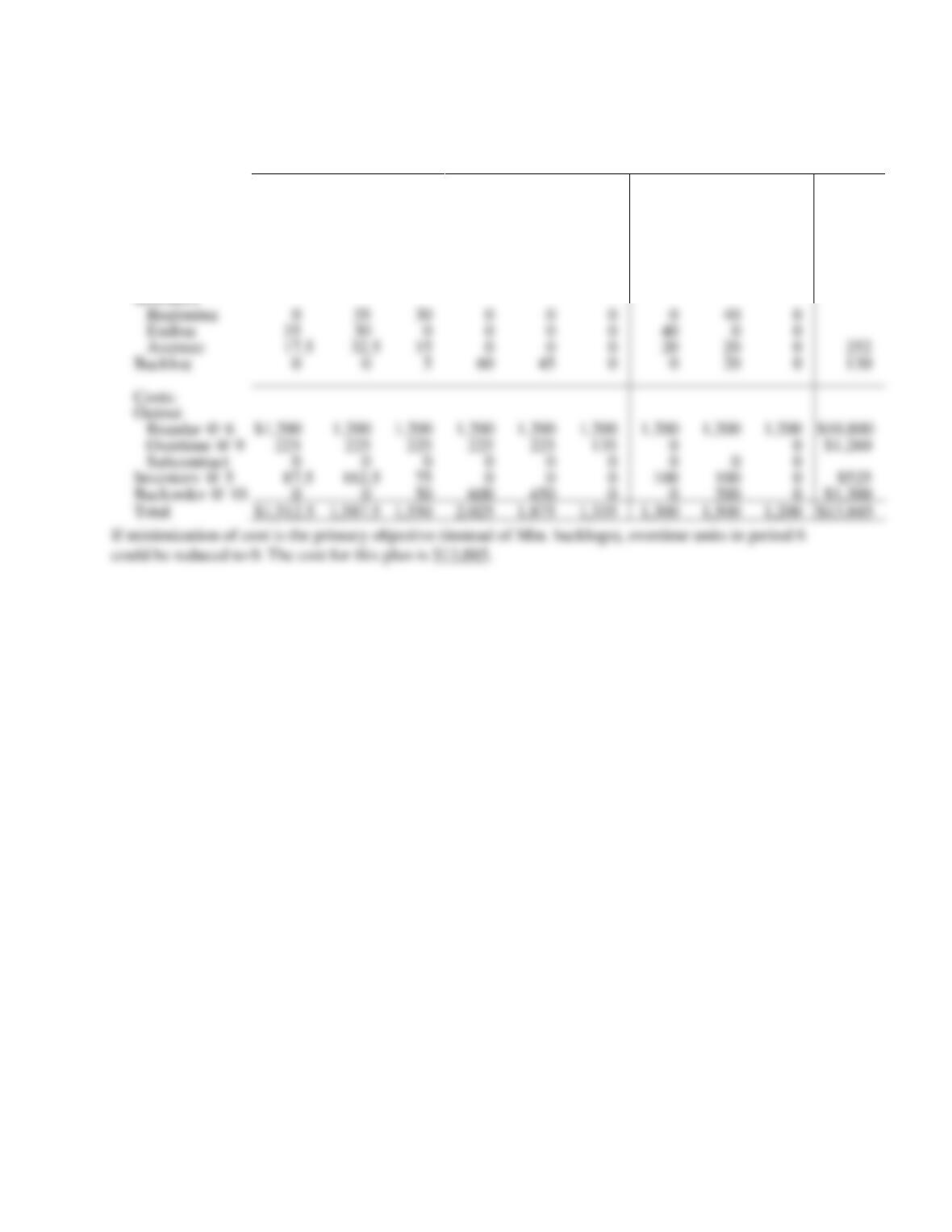
13. Several solutions are possible. Here is one.
Period
1
2
3
4
5
6
7
8
9
Total
Forecast
190
230
260
280
210
170
160
260
180
1,940
Output
Regular
210
210
210
210
210
180
180
180
180
1,770
Overtime
10
25
25
10
70
Costs:
Output
Regular @ 6
$1,260
1,260
1,260
1,260
1,260
1,080
1,080
1,080
1080
$10,620
Overtime @ 9
0
90
225
225
0
0
0
90
0
$630
Subcontract @ 8
0
160
160
160
0
0
160
160
0
$800
Hiring @ 200
200
0
0
0
0
0
0
0
0
$200
Layoff-firing @100
300
Inventory @ 5
125
137.5
150
125
0
Backorder @ 10
0
$0
Total
Subcontract
20
20
20
20
20
100
Output-
Forecast
20
10
0
10
40
0
Inventory
0
Ending
0
Average
0
Backlog
0
Chapter 11 – Aggregate Planning and Master Scheduling
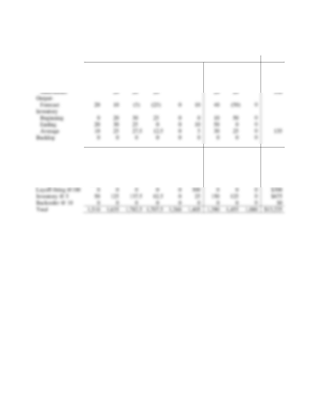
14.
–1
0
1
–91
Period
1
2
3
Unused Cap
Total
+1
Beg. Inv.
0
1
2
0
100
0
0
90
100
61
Reg.
60
61
62
0
1
450
50
0
30
500
81
Over.
80
81
82
0
0
50
0
10
50
91
Sub.
90
91
92
0
0
30
0
90
120
60
Reg.
63
60
61
0
2
4
500
0
31
500
80
Over.
83
80
81
0
4
50
0
11
50
90
Sub.
93
90
91
0
4
20
100
1
120
59
Reg.
66
63
60
0
3
8
4
500
32
500
79
Over.
86
83
80
0
8
4
50
12
50
89
Sub.
96
93
90
0
8
4
100
2
100
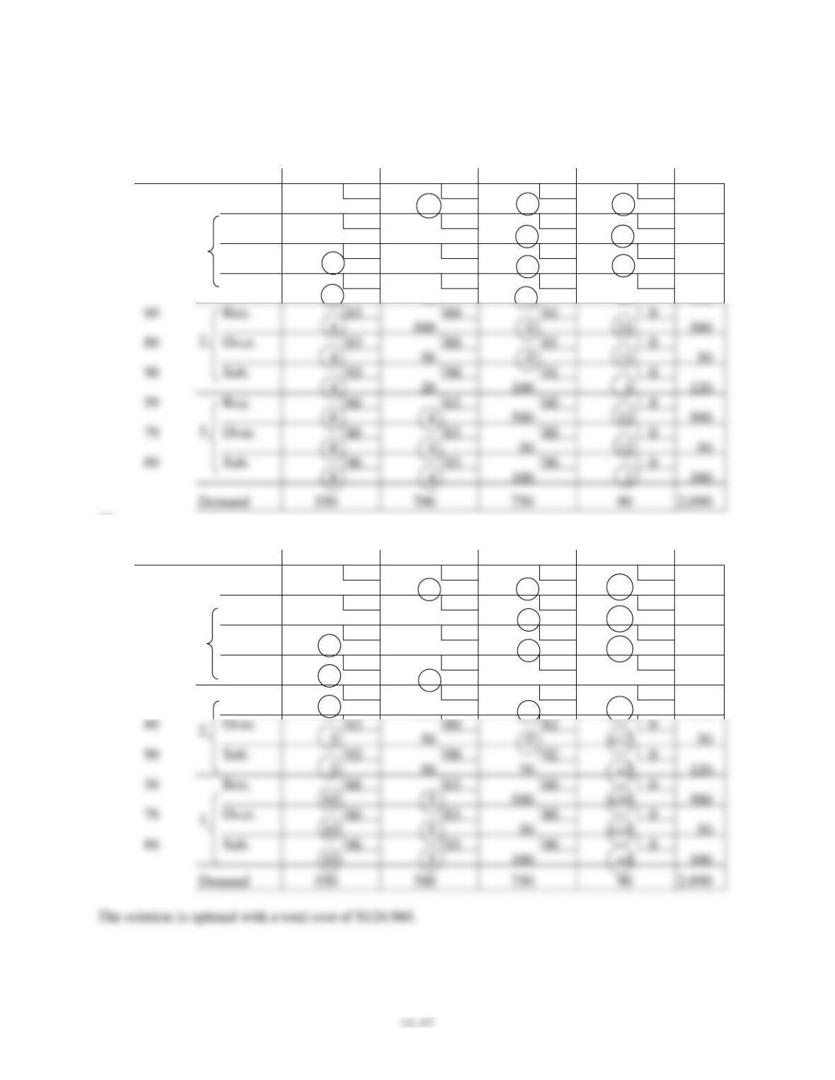
15.
–2
0
2
–92
Total
Period
1
2
3
4
Cap.
21
Beg. Inv.
0
2
4
0
100
0
0
+90
100
62
Reg.
60
62
64
0
1
450
50
0
+30
500
82
Over.
80
82
84
0
0
50
0
+10
50
92
Sub.
90
92
94
0
0
0
30
90
120
60
Reg.
63
60
62
0
2
80
Over.
83
80
82
0
5
50
0
+12
50
90
Sub.
93
90
92
0
5
50
70
120
58
Reg.
66
63
60
0
3
10
5
500
+34
500
78
Over.
86
83
80
0
10
5
50
+14
50
88
Sub.
96
93
90
0
10
5
100
100
5
500
0
+32
500
Chapter 11 – Aggregate Planning and Master Scheduling
11-18
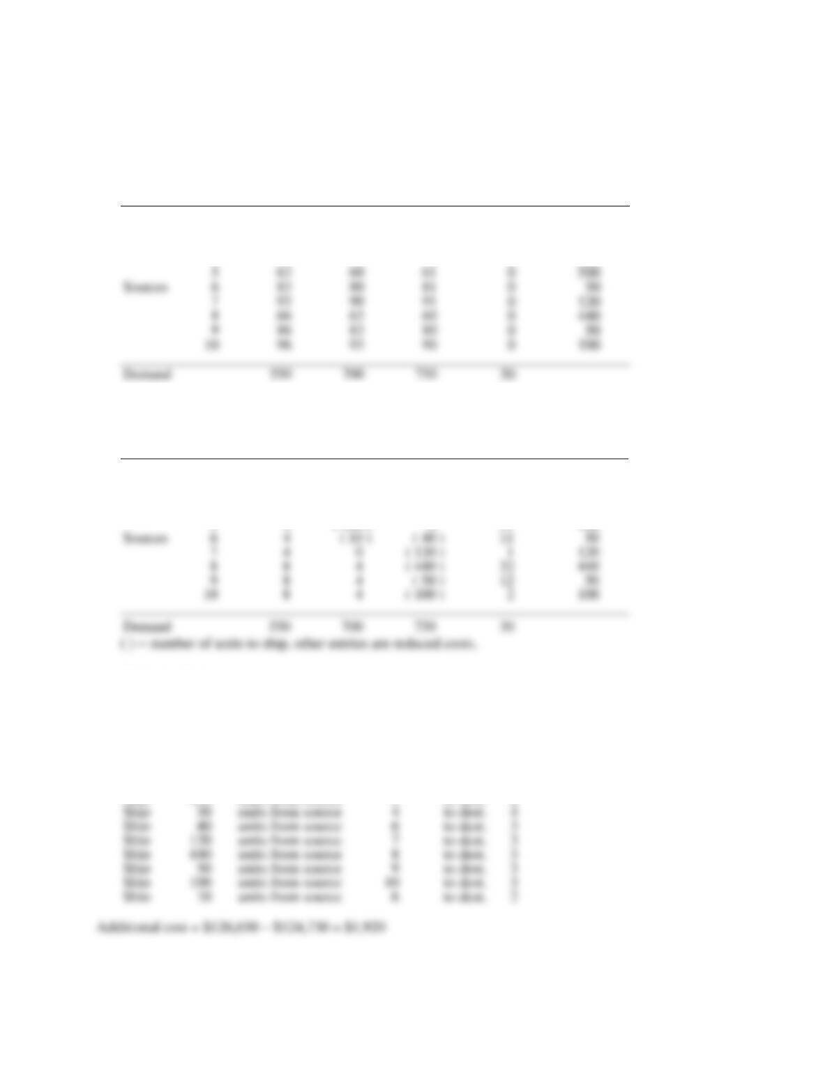
16.
Number of sources: 10
Number of destinations: 4
Destinations
1
2
3
4
Supply
1
0
1
2
0
100
2
60
61
62
0
500
3
80
81
82
0
50
4
90
91
92
0
120
Iteration: 3
Total cost: $126,650
Destinations
1
2
3
4
Supply
1
( 100 )
0
0
90
100
2
( 450 )
( 50 )
0
30
500
3
0
( 50 )
0
10
50
4
0
( 90 )
0
( 30 )
120
5
4
( 500 )
0
31
500
Sources
6
4
( 10 )
( 40 )
11
7
4
0
( 120 )
1
120
8
8
4
( 440 )
32
440
9
8
4
( 50 )
12
50
8
4
( 100 )
2
100
Demand
Optimal solution:
Iteration: 3
Total shipping cost : $126,650
Ship
100
units from source
1
to dest.
1
Ship
450
units from source
2
to dest.
1
Ship
50
units from source
2
to dest.
2
Ship
50
units from source
3
to dest.
2
Ship
90
units from source
4
to dest.
2
Ship
500
units from source
5
to dest.
2
Ship
30
units from source
4
to dest.
4
Ship
40
units from source
6
to dest.
3
Ship
120
units from source
7
to dest.
3
Ship
440
units from source
8
to dest.
3
Ship
50
units from source
9
to dest.
3
Ship
100
units from source
to dest.
3
Ship
10
units from source
6
to dest.
2
5
63
60
61
0
500
Sources
6
83
80
81
0
50
7
93
90
91
0
120
8
66
63
60
0
440
0
96
93
90
0
100
Demand
Chapter 11 – Aggregate Planning and Master Scheduling
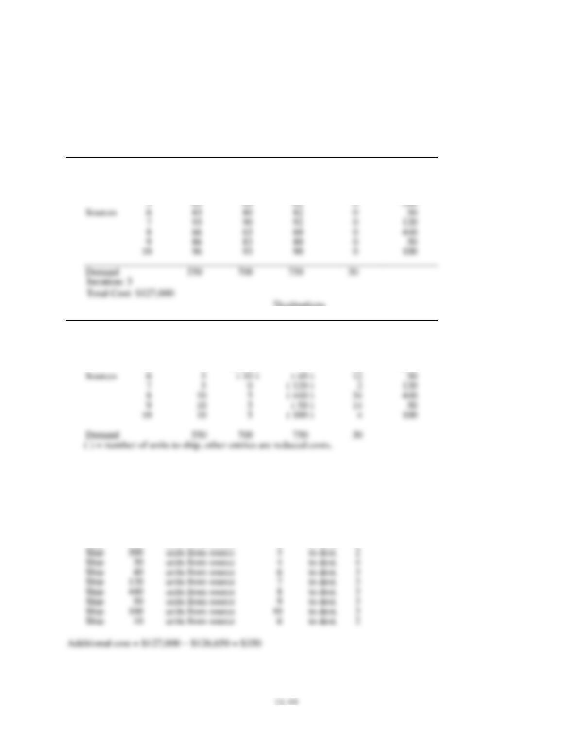
17.
Number of sources: 10
Number of destinations: 4
Destinations
1
2
3
4
Supply
1
0
2
4
0
100
2
60
62
64
0
500
3
80
82
84
0
50
4
90
92
94
0
120
5
63
60
62
0
500
Sources
6
83
80
82
0
50
7
93
90
92
0
120
8
66
63
60
0
440
9
86
83
80
0
50
96
93
90
0
100
Destinations
1
2
3
4
Supply
1
( 100 )
0
0
90
100
2
( 450 )
( 50 )
0
30
500
3
0
( 50 )
0
10
50
4
0
( 90 )
0
( 30 )
120
5
5
( 500 )
0
32
500
Sources
6
5
( 10 )
( 40 )
12
50
7
5
0
( 120 )
2
120
8
10
5
( 440 )
34
440
9
10
5
( 50 )
14
50
10
5
( 100 )
4
100
Demand
550
750
30
Optimal solution:
Iteration: 3
Total shipping cost: $127,00
Ship
100
units from source
1
to dest.
1
Ship
450
units from source
2
to dest.
1
Ship
50
units from source
2
to dest.
2
Ship
50
units from source
3
to dest.
2
Ship
90
units from source
4
to dest.
2
Ship
500
units from source
5
to dest.
2
Ship
30
units from source
4
to dest.
4
Ship
40
units from source
6
to dest.
3
Ship
120
units from source
7
to dest.
3
Ship
440
units from source
8
to dest.
3
Ship
50
units from source
9
to dest.
3
Ship
100
units from source
to dest.
3
Ship
10
units from source
6
to dest.
2
Chapter 11 – Aggregate Planning and Master Scheduling
11-20
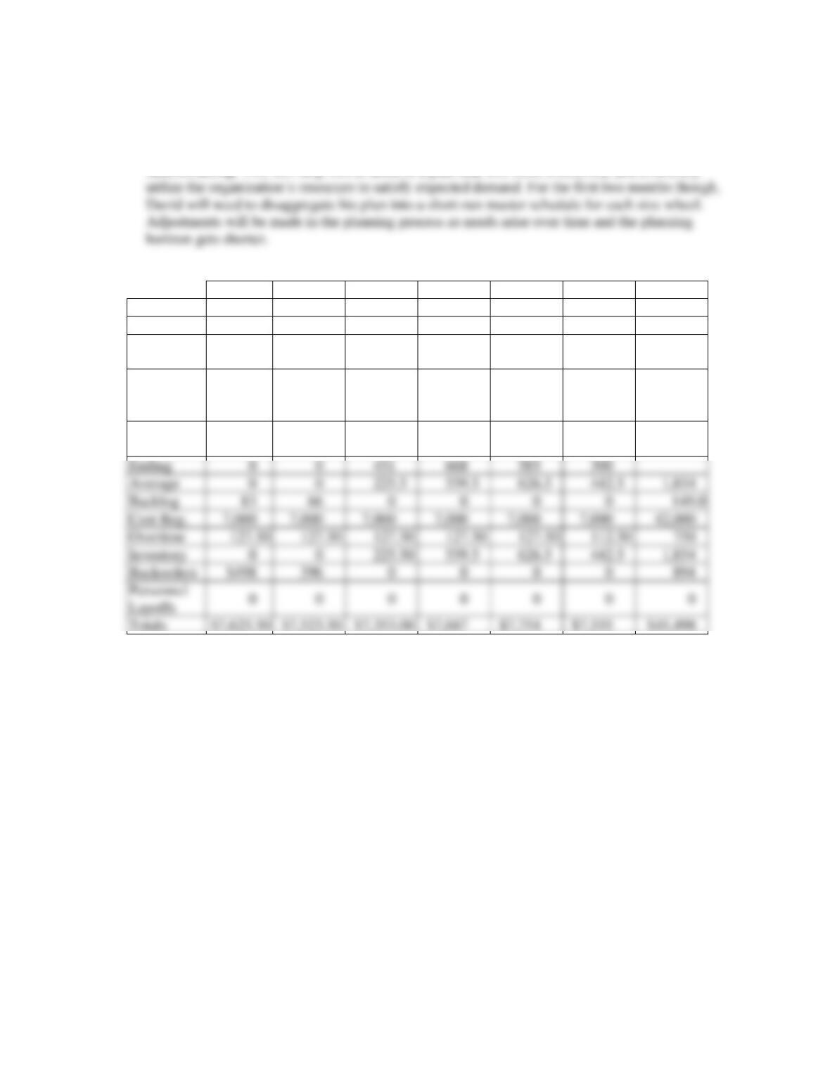
18. a. Initially, David should develop one aggregate plan for the next six months in order to determine
his output rate, employment levels and changes, inventory levels and changes, back orders, and
subcontracting. This will help him to achieve a plan that will more effectively and efficiently
b. and c.
Nov.
Dec.
Jan.
Feb.
Mar.
April
Total
Forecast
1,500
1,400
900
1,200
1,500
1,700
8,200
Output Reg.
1,400
1,400
1,400
1,400
1,400
1,400
8,400
Output
Overtime
17
17
17
17
17
15
100
Output
Minus
Forecast
-83
17
517
217
-83
-285
300
Inventory
Begin
0
0
0
451
668
585
Ending
Average
225.5
559.5
626.5
442.5
1,854
Backlog
149.0
Cost Reg.
42,000
Overtime
127.50
127.50
127.50
127.50
112.50
Backorders
396
Personnel
Layoffs
0
0
0
0
0
0
Totals
Chapter 11 – Aggregate Planning and Master Scheduling
11-21
19.
June
July
64
1
2
3
4
5
6
7
8
Forecast
30
30
30
30
40
40
40
40
Customer
33
20
10
4
2
ATP
31
36
68
70
70
Week
Inventory
From Pre-
vious Wk.
Requirements
Net
Inventories
Before MPS
(70) MPS
Projected
On-Hand
Inventory
1
64
33
31
–
31
2
31
30
1
70
71
3
71
30
41
–
41
4
41
30
11
–
11
5
11
40
70
41
6
41
40
70
71
7
71
40
–
31
8
31
40
70
61
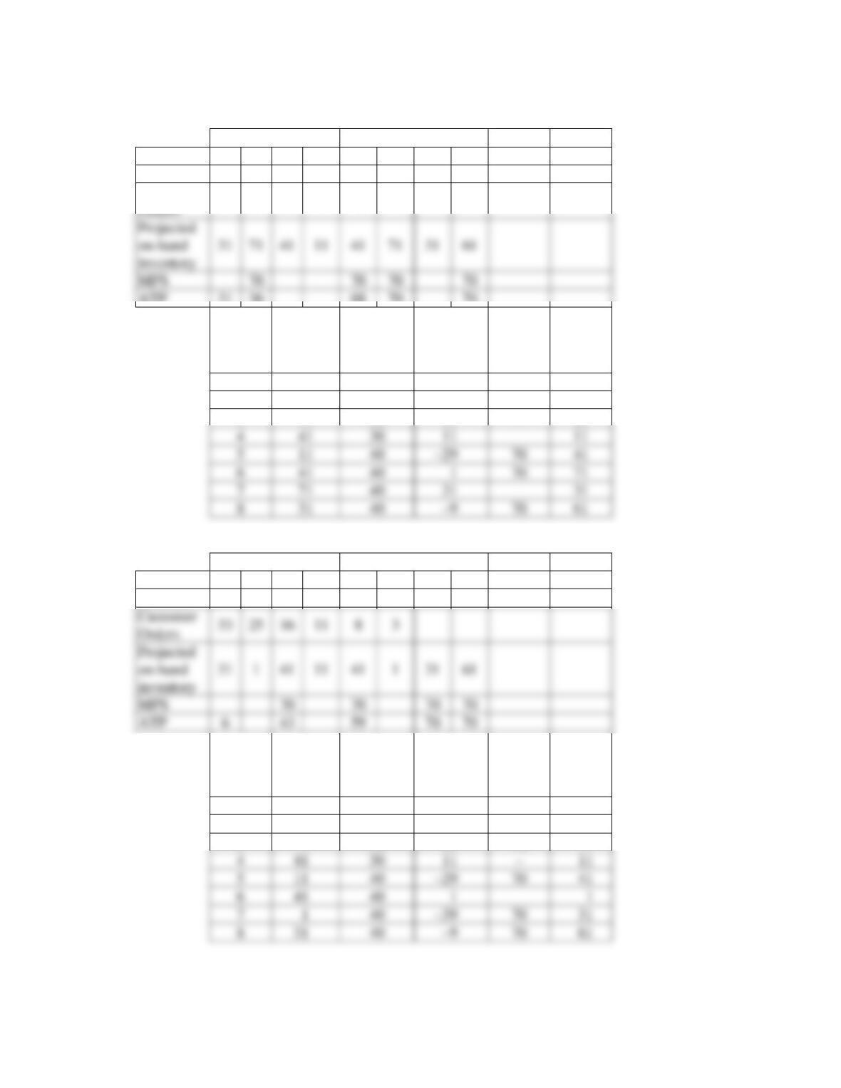
20.
June
July
64
1
2
3
4
5
6
7
8
Forecast
30
30
30
30
40
40
40
40
Customer
33
25
16
8
3
MPS
70
70
70
70
ATP
6
43
59
70
70
Week
Inventory
From Pre-
vious Wk.
Requirements
Net
Inventories
Before MPS
(70) MPS
Projected
On-Hand
Inventory
1
64
33
31
–
31
2
31
30
1
–
1
3
1
30
–29
70
41
4
41
30
–
5
11
40
–29
70
41
6
41
40
7
1
40
70
8
31
40
70
61
MPS
70
70
70
70
Chapter 11 – Aggregate Planning and Master Scheduling
11-22
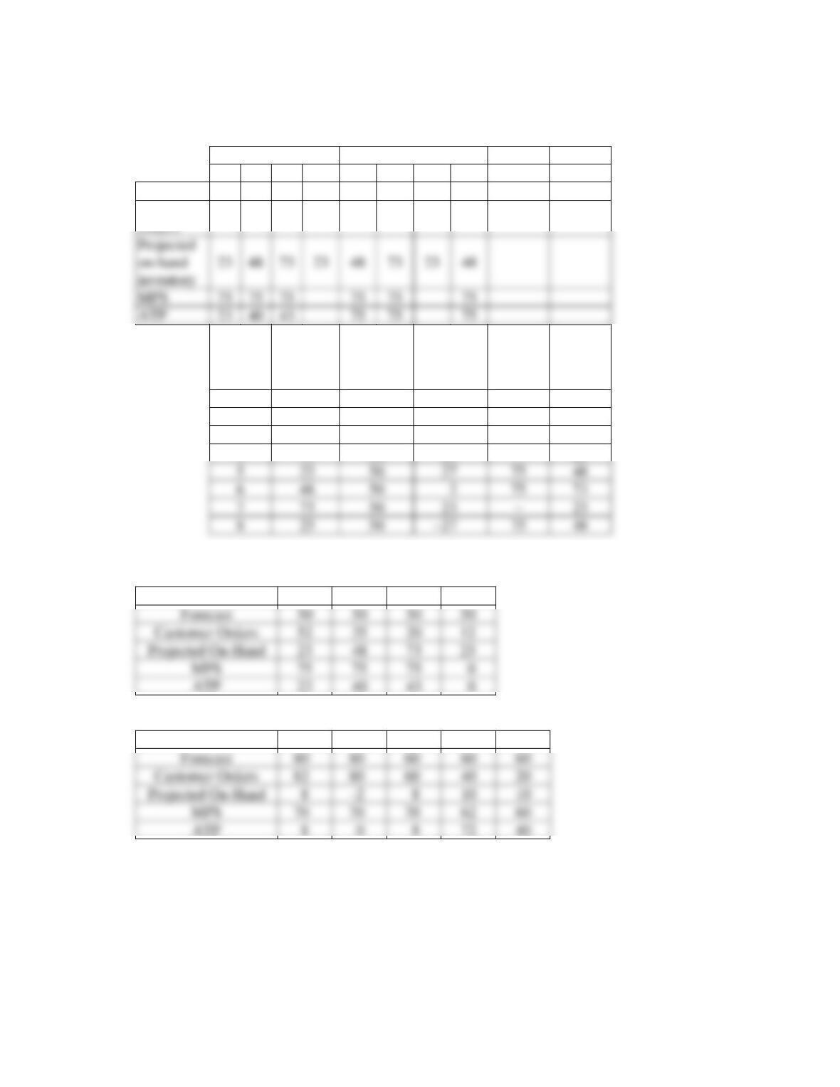
21.
June
July
1
2
3
4
5
6
7
8
Forecast
50
50
50
50
50
50
50
50
Customer
52
35
20
12
Week
Inventory
From Pre-
vious Wk.
Requirements
Net
Inventories
Before MPS
(70) MPS
Projected
On-Hand
Inventory
1
0
52
–52
75
23
2
23
50
–27
75
48
3
48
50
–2
75
73
4
73
50
23
–
23
5
23
50
–27
75
48
6
48
50
–2
75
73
7
73
50
23
–
23
8
23
50
–27
75
48
22. Starting Inventory = 0 units
Period
1
2
3
4
23. Starting Inventory = 20 units
Period
1
2
3
4
5
8
8
Orders
on-hand
MPS
75
75
75
ATP
75
75
75
Chapter 11 – Aggregate Planning and Master Scheduling
11-23
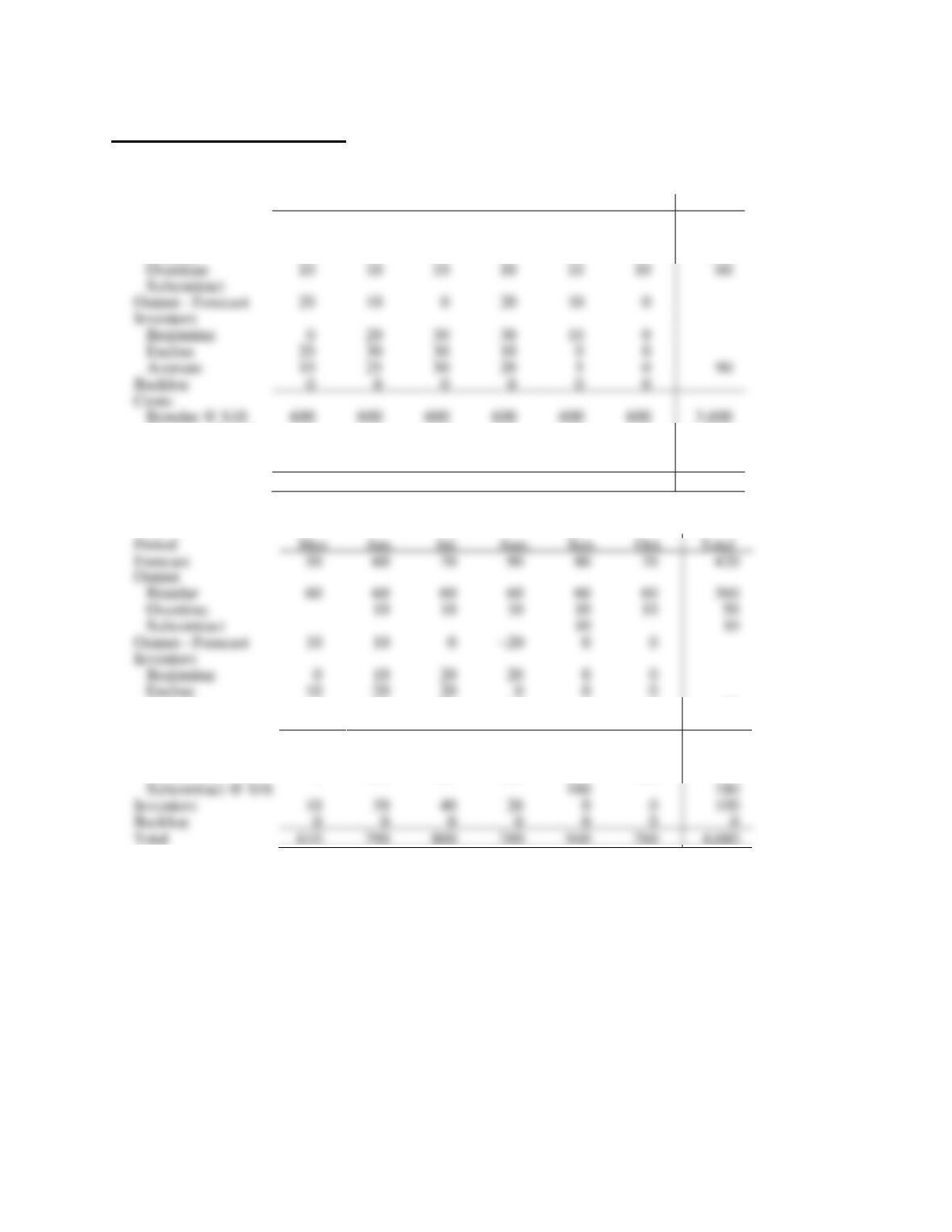
Case: Eight Glasses a Day
1. Strategy 1: Level production supplemented by up to 10 tank loads a month from overtime.
Period
May
Jun.
Jul.
Aug.
Sep.
Oct.
Total
Forecast
50
60
70
90
80
70
420
Output
Regular
60
60
60
60
60
60
360
Overtime @ $16
160
160
160
160
160
160
960
Inventory
20
50
60
40
10
0
180
Backlog
0
0
0
0
0
0
0
Total
780
810
820
800
770
760
4,740
Strategy 2: A combination of overtime, inventory and subcontracting.
Period
May
Jul.
Aug.
Sep.
Oct.
Total
Forecast
50
60
70
90
80
70
420
Output
Regular
60
60
60
60
60
60
360
Overtime
10
10
10
10
10
50
Subcontract
10
10
Output – Forecast
10
10
0
0
0
Inventory
Beginning
0
10
20
20
0
0
Ending
10
20
20
0
0
0
Average
5
15
20
10
0
0
50
Backlog
0
0
0
0
0
0
0
Costs:
Regular @ $10
600
600
600
600
600
600
3,600
Overtime @ $16
0
160
160
160
160
160
800
Subcontract @ $18
180
180
Inventory
10
30
40
20
0
0
100
Backlog
0
0
0
0
0
0
0
Total
610
790
800
780
940
760
4,680
Overtime
10
10
10
10
10
10
60
Subcontract
20
10
0
0
Inventory
Beginning
0
20
30
30
10
0
Ending
20
30
30
10
0
0
Average
10
25
30
20
5
0
90
Backlog
0
0
0
0
0
0
Costs:
Regular @ $10
Chapter 11 – Aggregate Planning and Master Scheduling
11-24
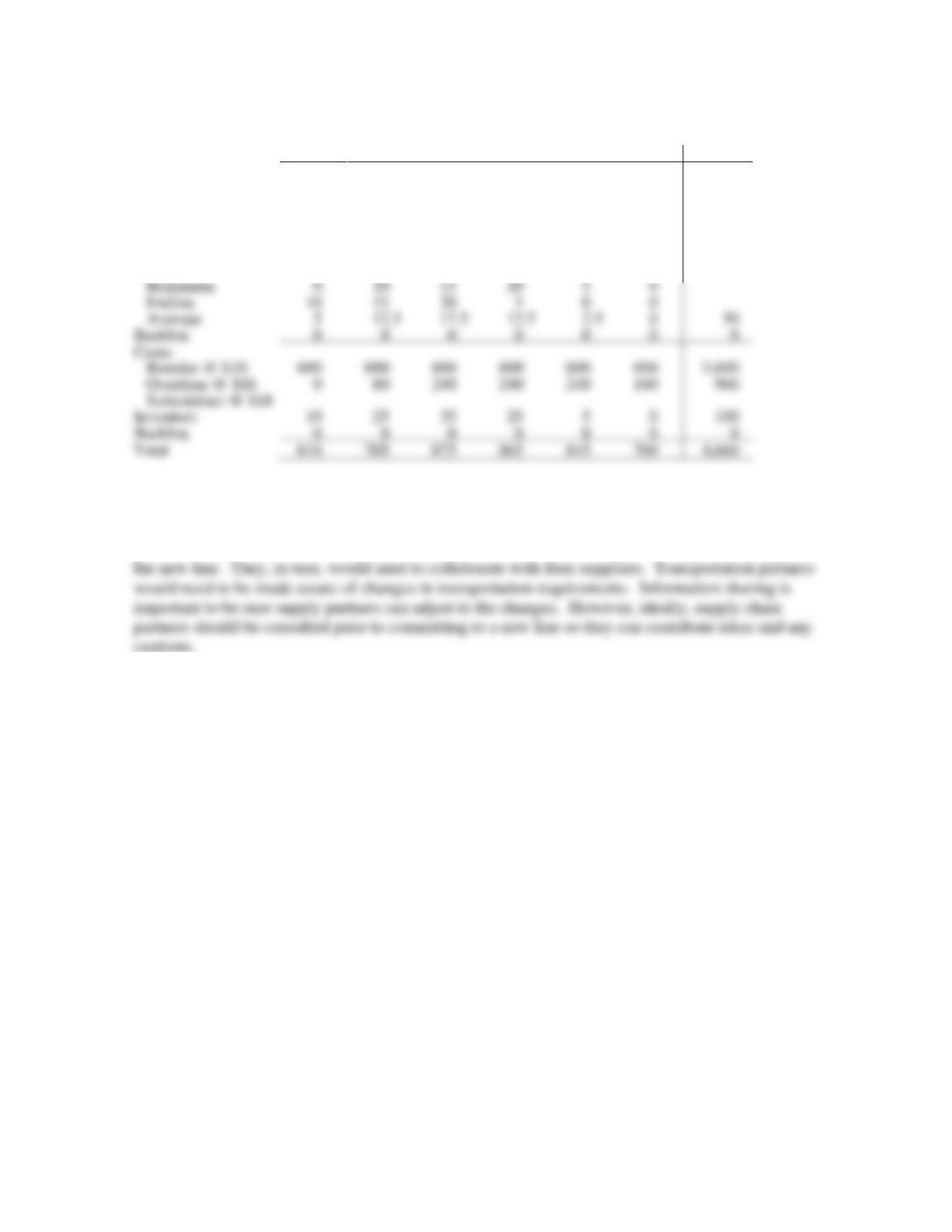
Strategy 3: Using inventory up to 15 tank loads a month from overtime.
Period
May
Jun.
Jul.
Aug.
Sep.
Oct.
Total
Forecast
50
60
70
90
80
70
420
Output
Regular
60
60
60
60
60
60
360
Overtime
5
15
15
15
10
60
Subcontract
Output – Forecast
10
5
5
–15
–5
0
Inventory
Since $4,660 < $4,680 < $4,740, the company should choose the third strategy.
2. Suppliers would need to know projections of initial demand and demand growth over time, and
product characteristics that would relate to new materials and new methods so they could prepare for
Beginning
0
10
15
20
5
0
Ending
10
15
20
Average
5
12.5
17.5
12.5
2.5
0
50
Backlog
Regular @ $10
Overtime @ $16
0
80
240
240
240
160
Subcontract @ $18
Inventory
10
25
35
25
5
0
Backlog