Chapter 11
Integer Linear Programming
Learning Objectives
1. Be able to recognize the types of situations where integer linear programming problem formulations
are desirable.
5. See how zero-one integer linear variables can be used to handle special situations such as multiple
choice, k out of n alternatives, and conditional constraints.
6. Be familiar with the computer solution of MILPs.
7. Understand the following terms:
all-integer mutually exclusive constraint
mixed integer k out of n alternatives constraint
Chapter 11
17 – 2
Solutions:
1. a. This is a mixed integer linear program. Its LP Relaxation is
Max
30x1
+
25x2
s.t.
x1, x2 0
b. This is an all-integer linear program. Its LP Relaxation just requires dropping the words “and
integer” from the last line.
2. a.
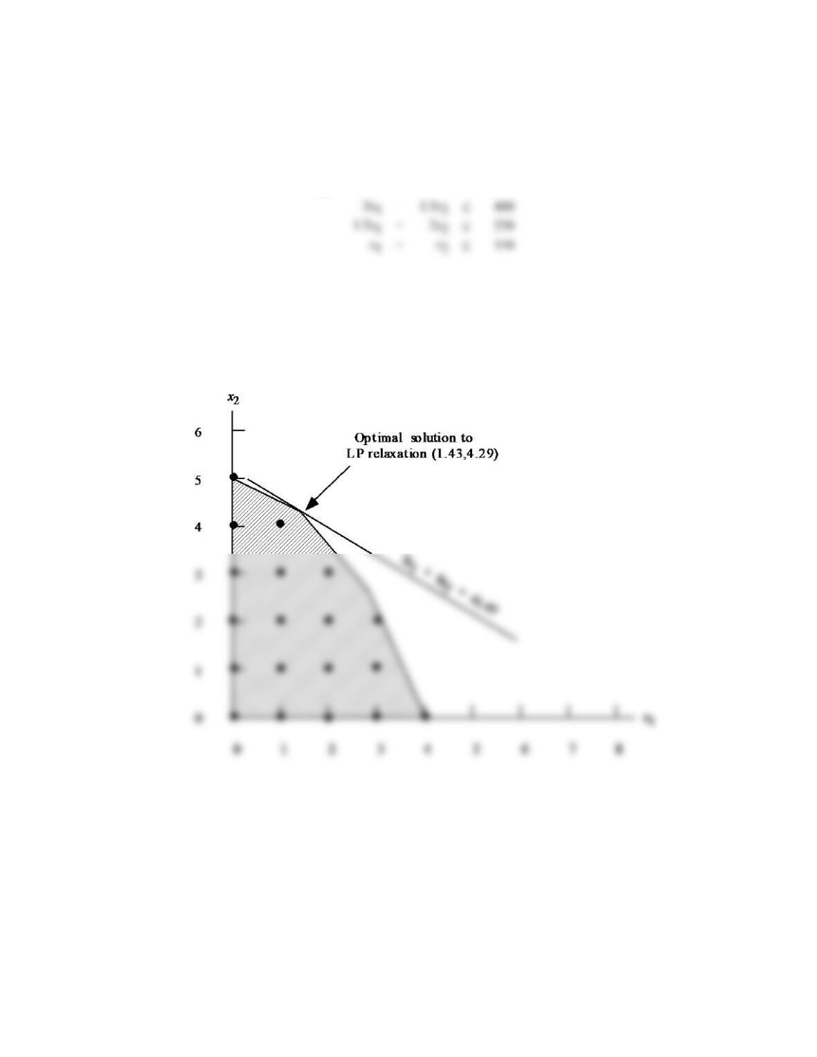
b. The optimal solution to the LP Relaxation is given by x1 = 1.43, x2 = 4.29 with an objective function
value of 41.47.
Rounding down gives the feasible integer solution x1 = 1, x2 = 4. Its value is 37.
17 – 3
c.
3
4
5
6 Opt imal Integer Solut ion
x2
5x1 + 8 x2 = 40
(0,5 )
3. a.
Chapter 11
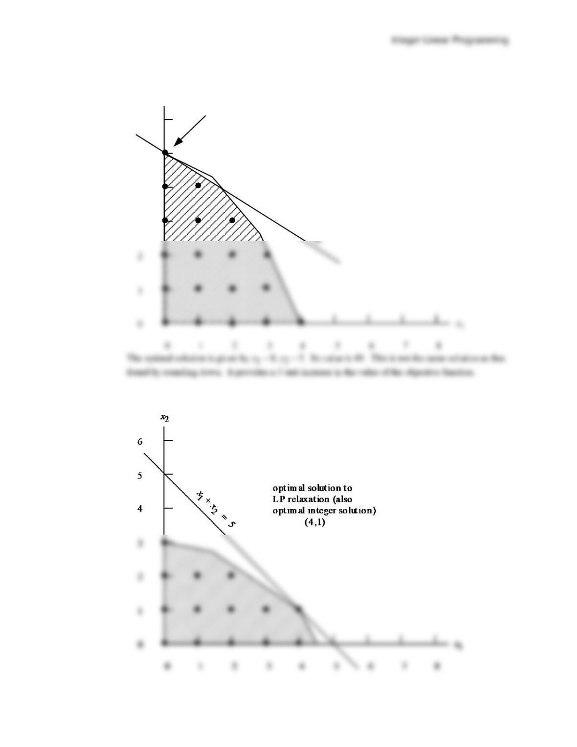
b. The optimal solution to the LP Relaxation is shown on the above graph to be x1 = 4, x2 = 1. Its
value is 5.
4. a.
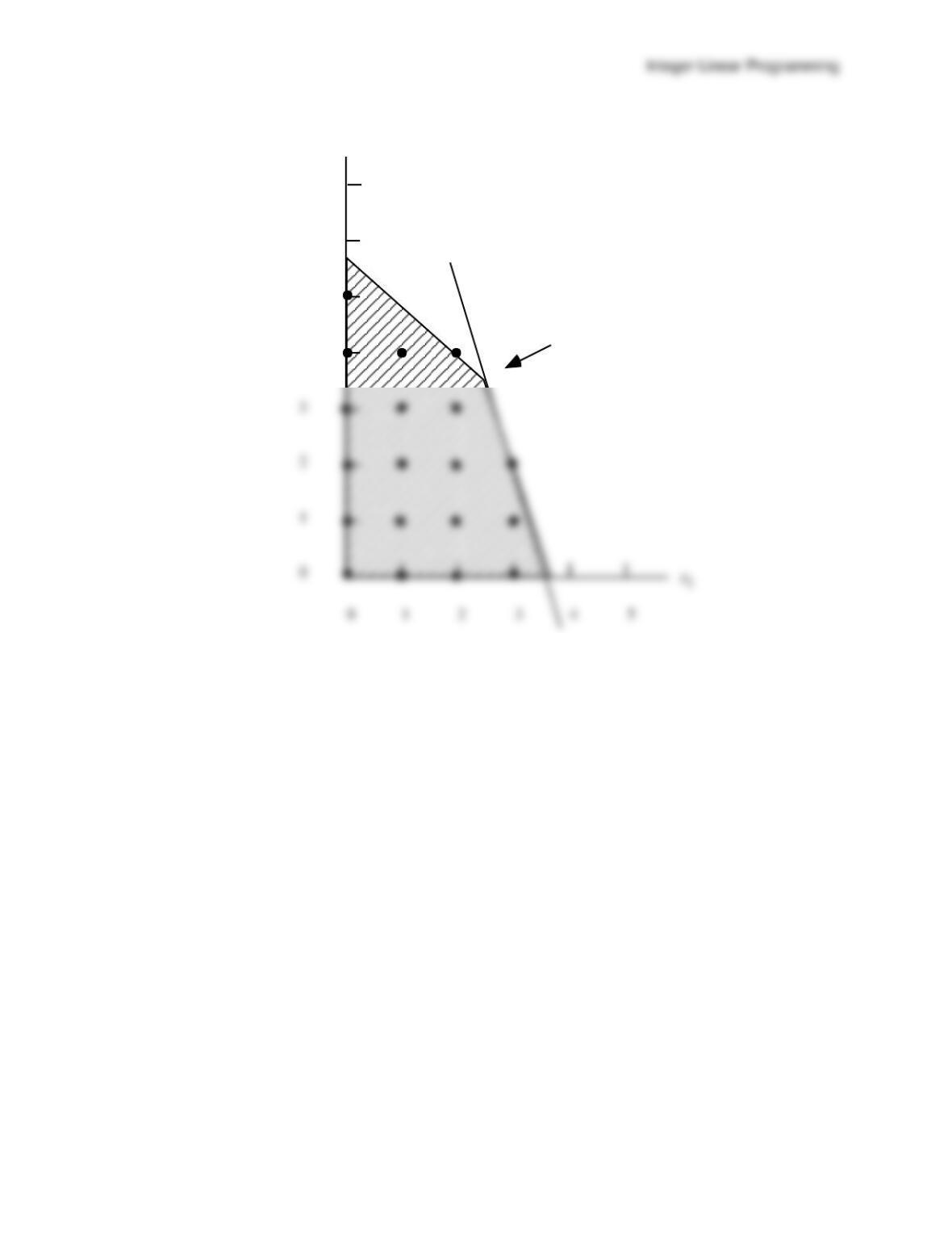
The value of the optimal solution to the LP Relaxation is 36.7 and it is given by x1 = 3.67, x2 = 0.0.
Since we have all less-than-or-equal-to constraints with positive coefficients, the solution obtained
by “rounding down” the values of the variables in the optimal solution to the LP Relaxation is
feasible. The solution obtained by rounding down is x1 = 3, x2 = 0 with value 30.
17 – 5
b.
4
5
6
7
10 x1 + 3 x2 = 36
x2
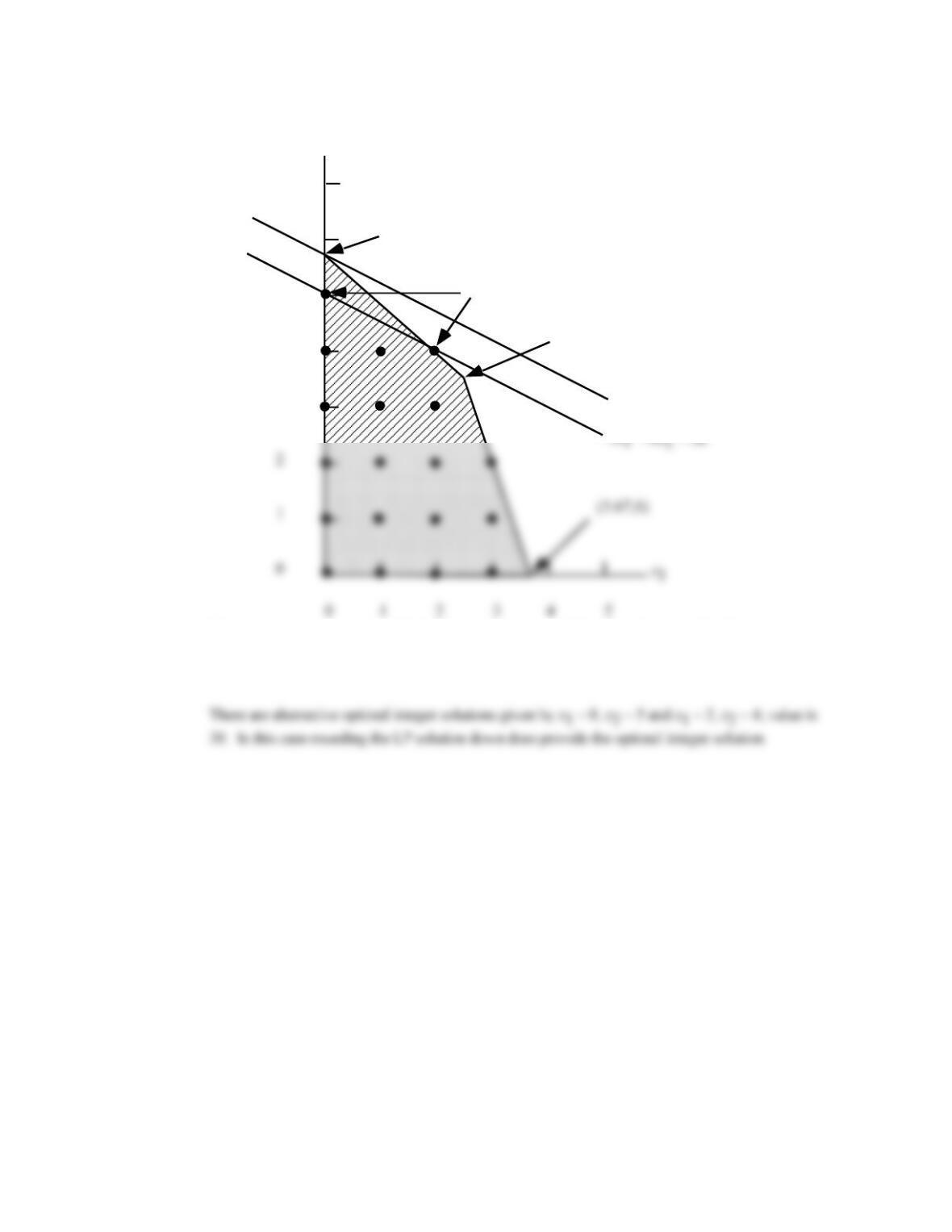
The optimal solution to the ILP is given by x1 = 3, x2 = 2. Its value is 36. The solution found by
“rounding down” the solution to the LP relaxation had a value of 30. A 20% increase in this value
was obtained by finding the optimal integer solution – a substantial difference if the objective
function is being measured in thousands of dollars.
Chapter 11
17 – 6
c.
..
3
4
5
6
7
Optimal solution to
LP relaxation (0,5.71)
Optimal integer solutions
(2.47,3.60)
3x1 + 6x2 = 34.26
x2
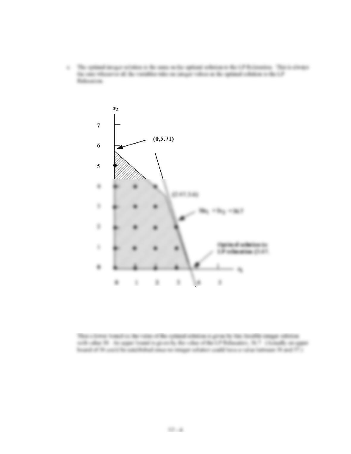
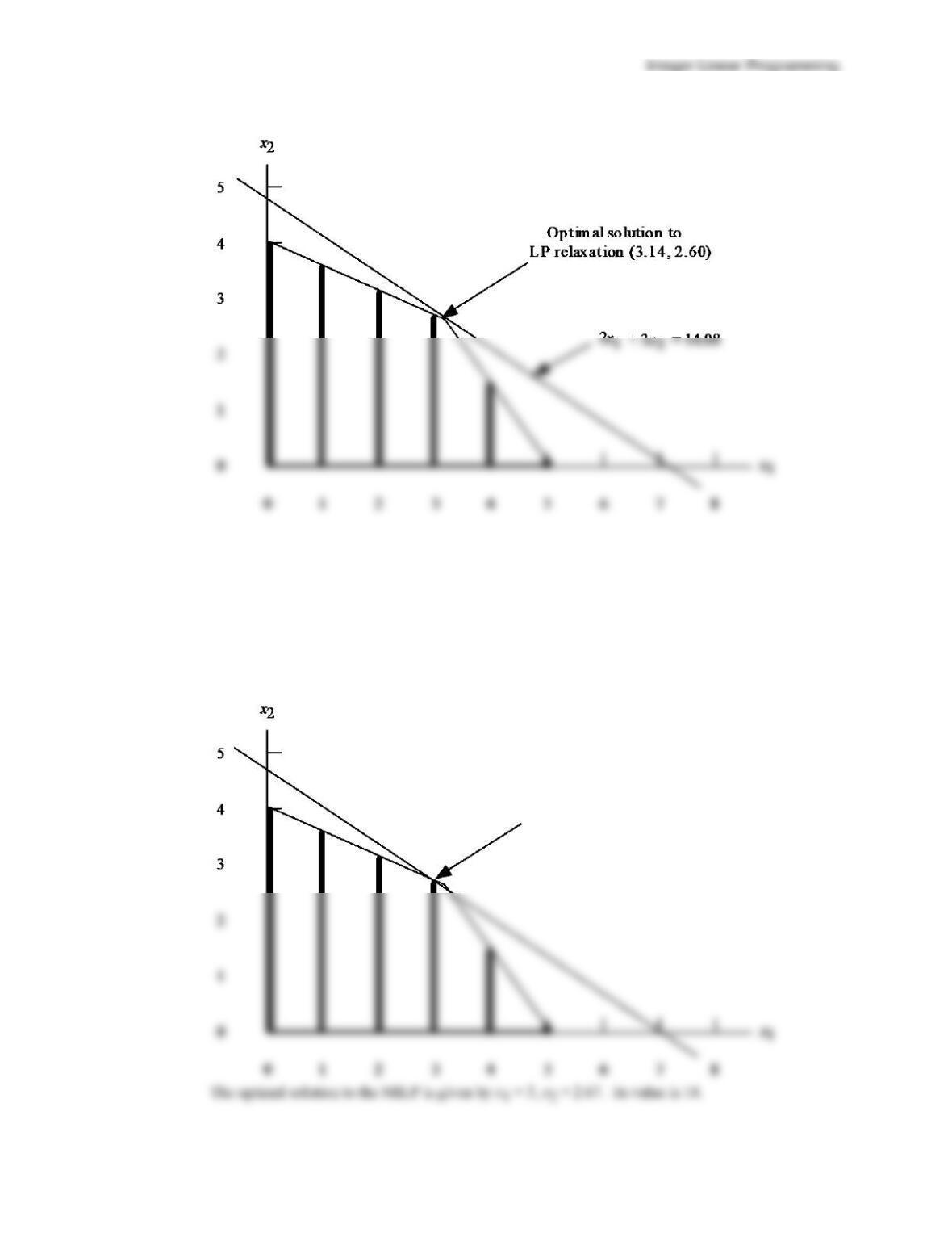
The optimal solution to the LP Relaxation is x1= 0, x2 = 5.71 with value = 34.26. The solution
obtained by “rounding down” is x1 = 0, x2 = 5 with value 30. These two values provide an upper
bound of 34.26 and a lower bound of 30 on the value of the optimal integer solution.
17 – 7
5. a.
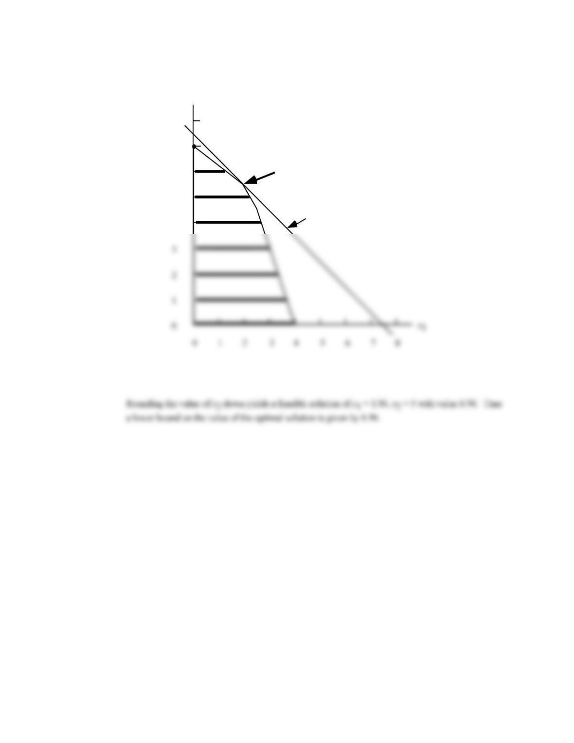
The feasible mixed integer solutions are indicated by the boldface vertical lines in the graph above.
b. The optimal solution to the LP relaxation is given by x1 = 3.14, x2 = 2.60. Its value is 14.08.
Rounding the value of x1 down to find a feasible mixed integer solution yields x1 = 3, x2 = 2.60 with
a value of 13.8. This solution is clearly not optimal. With x1 = 3 we can see from the graph that x2
can be made larger without violating the constraints.
c.
Optimal mixed integer
solution (3, 2.67)
Chapter 11
17 – 8
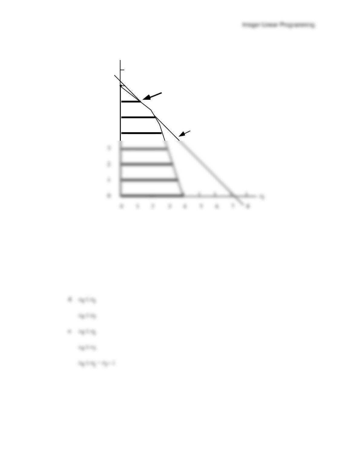
6. a.
4
5
6
7
8
Opt imal solution to
LP relaxat ion (1.96, 5.48)
x2
x1 + x2 = 7.44
b. The optimal solution to the LP Relaxation is given by x1 = 1.96, x2 = 5.48. Its value is 7.44. Thus
an upper bound on the value of the optimal is given by 7.44.
17 – 9
c.
Optim al mixed int eger
solution (1.29, 6 )
4
5
6
7
8
x2
x1 + x2 = 7 .2 9
The optimal solution to the MILP is x1 = 1.29, x2 = 6. Its value is 7.29.
The solution x1 = 2.22, x2 = 5 is almost as good. Its value is 7.22.
7. a. x1 + x3 + x5 + x6 = 2
b. x3 – x5 = 0
c. x1 + x4 = 1
Chapter 11
17 – 10
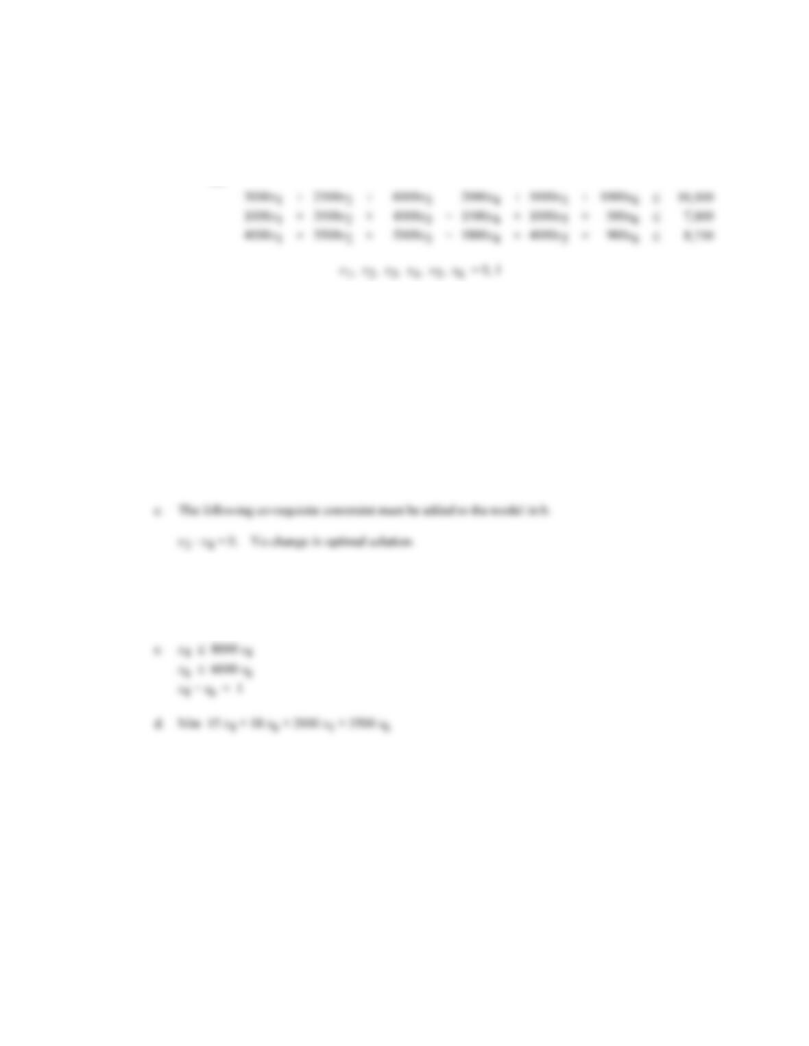
8. a. Let
1 if investment alternative is selected
0 otherwise
i
i
x
=
max
4000x1
+
6000x2
+
10500x3
+
4000x4
+
8000x5
+
3000x6
3000x1
2500x2
2000x4
5000x5
1000x6
1000x1
+
3500x2
+
+
1500x4
+
1000x5
+
4000x1
+
3500x2
+
+
1800x4
+
4000x5
+
The optimal solution is
x3 = 1
x4 = 1
x6 = 1
Value = 17,500
b. The following mutually exclusive constraint must be added to the model.
x1 + x2 1 No change in optimal solution.
9. a. x4 8000 s4
b. x6 6000 s6
Integer Linear Programming
17 – 11
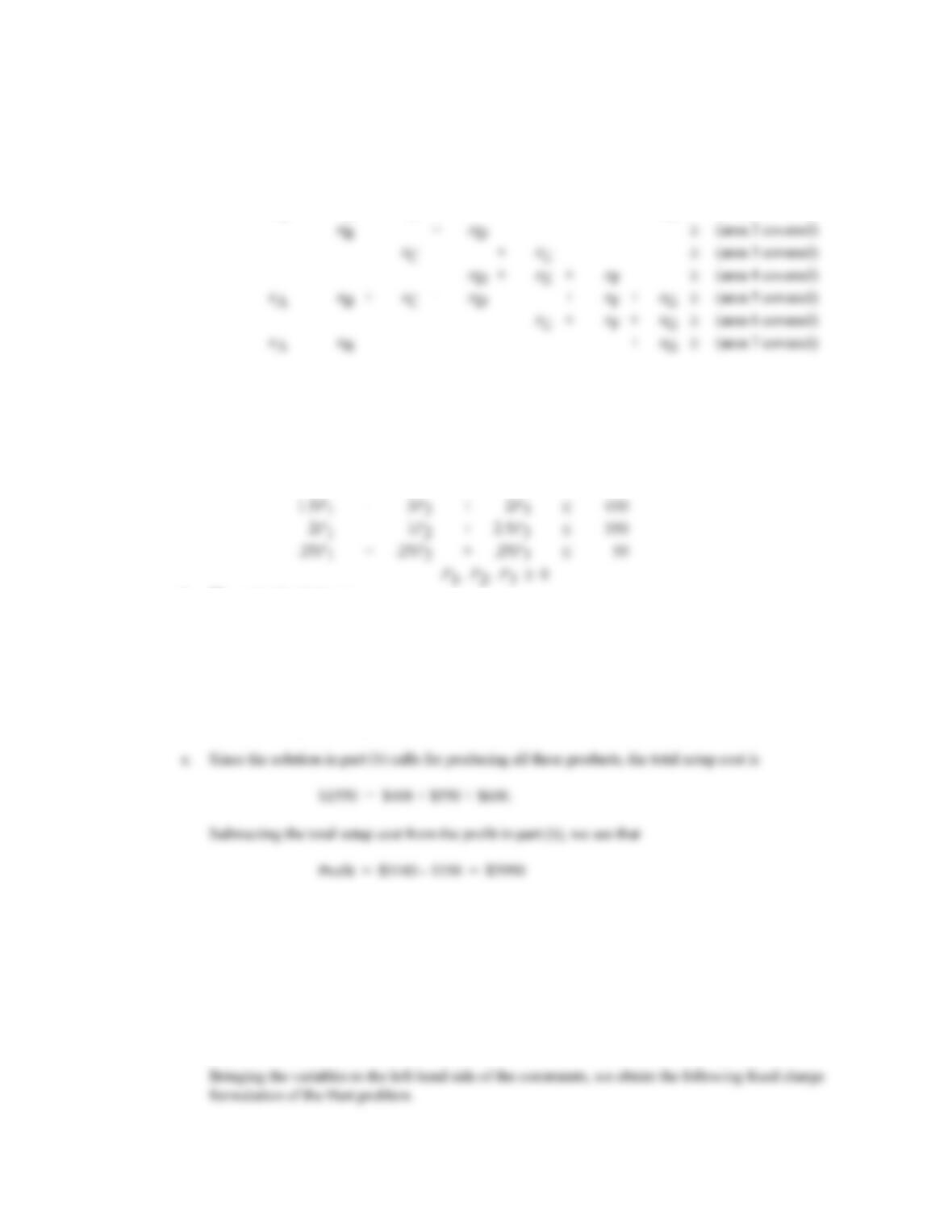
10. a. Let xi = 1 if a substation is located at site i, 0 otherwise
min
xA
+
xB
+
xC
+
xD
+
xE
+
xF
+
xG
s.t.
xA
+
xB
+
xC
+
xG
1 (area 1 covered)
xB
xD
1 (area 2 covered)
xC
+
xE
xD
+
xE
xF
1 (area 4 covered)
xA
+
xB
+
xC
xD
xF
+
xG
1 (area 5 covered)
xE
+
xF
+
xG
xA
+
xB
+
xG
1 (area 7 covered)
b. Choose locations B and E.
11. a. Let Pi = units of product i produced
Max
25P1
+
28P2
+
30P3
s.t.
+
+
+
+
b. The optimal solution is
P1 = 60
P2 = 80 Value = 5540
P3 = 60
This solution provides a profit of $5540.
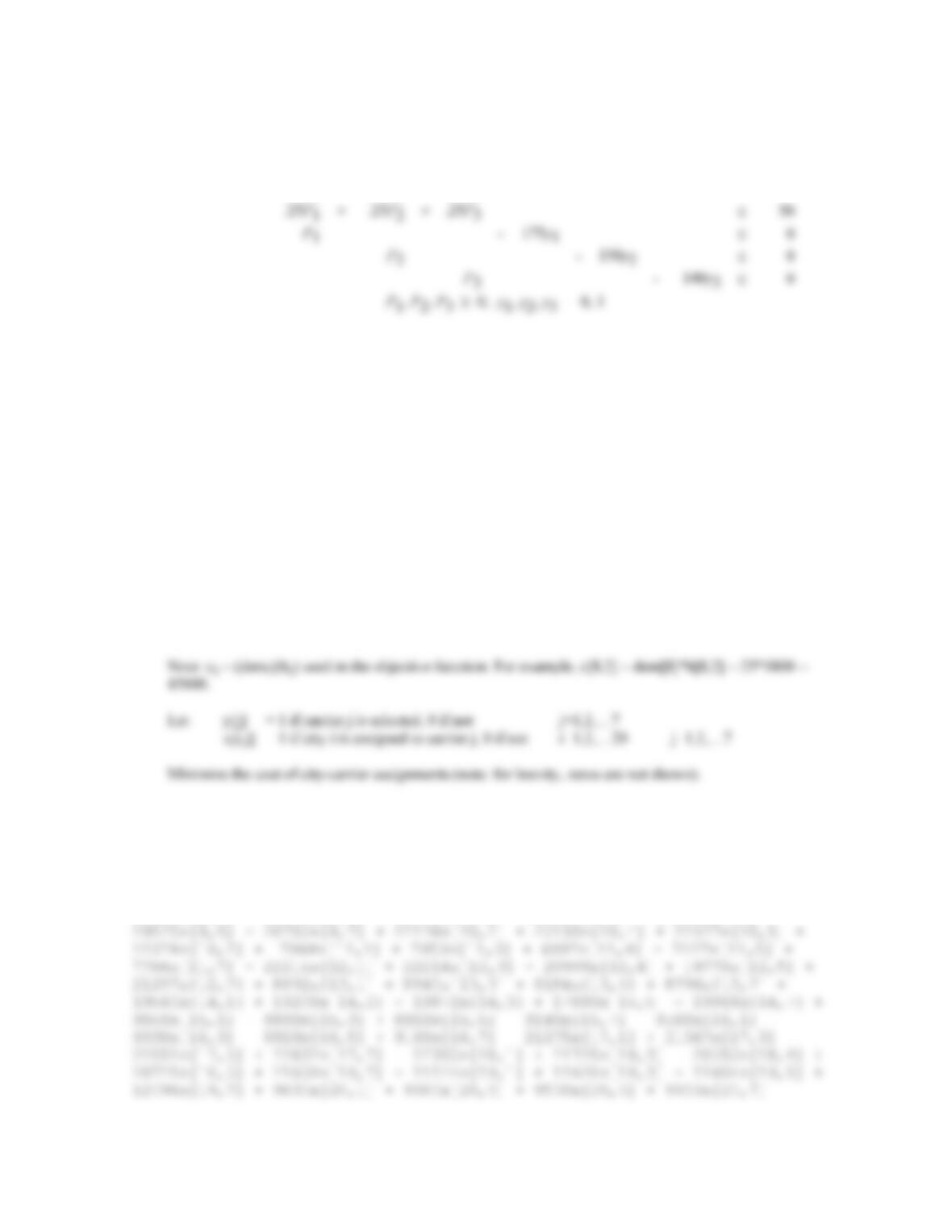
d. We introduce a 0-1 variable yi that is one if any quantity of product i is produced and zero otherwise.
With the maximum production quantities provided by management, we obtain 3 new constraints:
P1 175y1
P2 150y2
P3 140y3
Chapter 11
17 – 12
Max
25P1
+
28P2
+
30P3
–
400y1
–
550y2
–
600y3
s.t.
1.5P1
+
3P2
+
2P3
450
2P1
+
1P2
+
2.5P3
350
.25P1
+
+
.25P3
–
175y1
–
150y2
–
140y3
e. The optimal solution is
P1 = 100 y1 = 1
P2 = 100 y2 = 1 Value = 4350
P3 = 0 y3 = 0
The profit associated with this solution is $4350. This is an improvement of $360 over the solution
in part (c).
12. a.
We use the following data:
b[i,j] = the bid for city i from carrier j, i=1,2,…20 j=1,2,…7
dem[i] = the demand in truckloads for city i i=1,2,…20
c[i,j] = the cost of assigning city i to carrier j i=1,2,…20 j=1,2,…7
Minimize
65640x[1,5] + 49980x[1,6] + 53700x[1,7] + 14530x[2,2] + 26020x[2,5] +
17670x[2,6] + 30680x[3,2] + 45660x[3,5] + 37140x[3,6] + 37400x[3,7] +
67480x[4,2] + 104680x[4,5] + 69520x[4,6] + 15230x[5,2] + 22390x[5,5] +
17710x[5,6] + 18550x[5,7] + 15210x[6,2] + 15710x[6,5] + 15450x[6,7] +
25200x[7,2] + 23064x[7,4] + 23256x[7,5] + 24600x[7,7] + 45000x[8,2] +
35800x[8,4] + 35400x[8,5] + 43475x[8,7] + 28350x[9,2] + 30825x[9,4] +