Step 3. Analyze f“(x):
f“(x) =
22 2
24
2(1)4(1)(2)
(1 )
x
xx x
x
=
222
24
2(1)[(1)4]
(1 )
x
xx
x
=
2
23
2(1 3 )
(1 )
x
x
3Concave
Graph
Concave
Concave
3
2
02()
x
Step 4. Sketch the graph of f:
1
2
31
2
()
1
1
x
fx
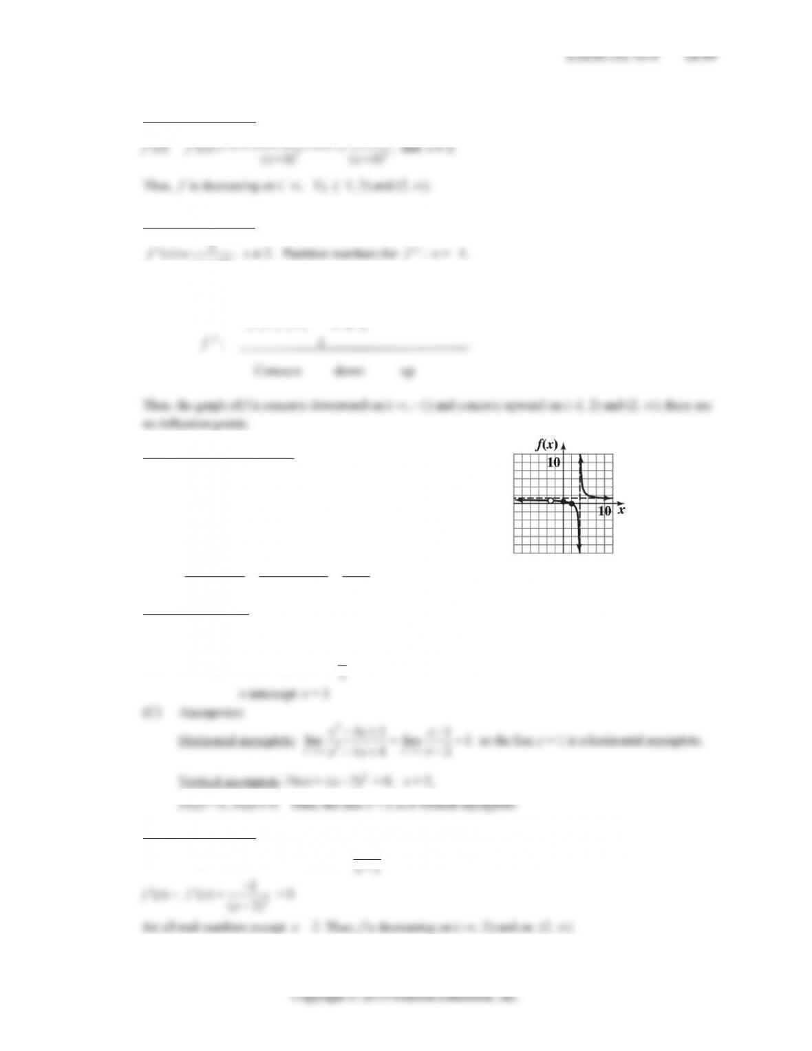
40. f(x) = 2
2
9
x
x
Step 1. Analyze f(x):
(A) Domain: All real numbers except x = –3, x = 3.
(B) Intercepts: y-intercept: f(0) = 0
2
x
x
11-42 CHAPTER 11: GRAPHING AND OPTIMIZATION
Step 2. Analyze f ꞌ(x):
222
2( 9) 2(2) 2 18 4
(9) (9)
x
xx x x
xx
2
2( 9)
(9)
x
x
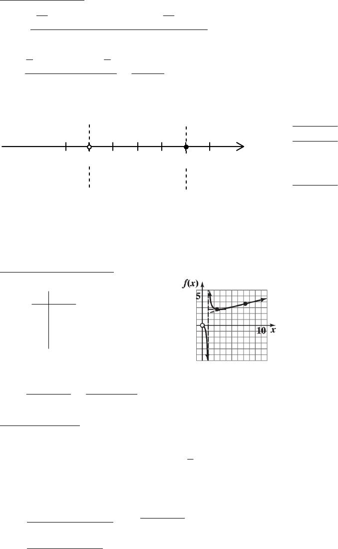
Critical values: None
Partition numbers: x = –3, x = 3
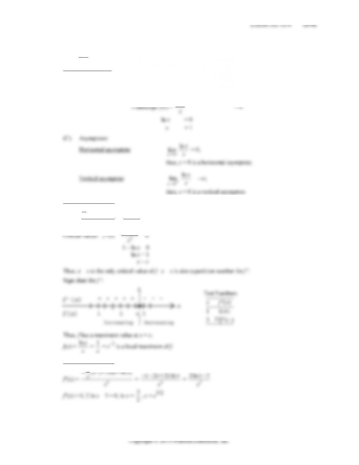
Sign chart for f ꞌ:
Test Numbers
Step 3. Analyze f“(x):
f“(x) = –2{2x(x2 – 9)–2 – 4x(x2 – 9)–3(x2 + 9)}
2
24(9)
xxx
22
2( 9) 4( 9)
xx xx
Sign chart for f“:
x
– – + + + – – – + +
ND
ND
f“(x)
0
Test Numbers
688
343
“( )
4()
x
fx
Step 4. Sketch the graph of f:
8
()
x
fx
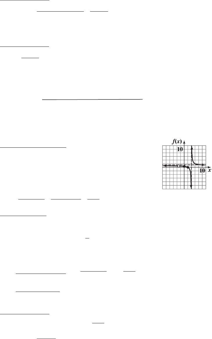
42. f(x) = 2
(2)
x
x
Step 1. Analyze f(x):
EXERCISE 11-4 11-43
(B) Intercepts: y-intercept: f(0) = 0
(C) Asymptotes:
Step 2. Analyze f ꞌ(x):
f ꞌ(x) =
2
(2)2(2) 22 (2)
xxxxxx
0ND Test Numbers
Step 3. Analyze f“(x):
(2) (2)
xx
Partition numbers for f“: x = –4, x = 2
Sign chart for f“:
-5 -4 3
2
0
1
0()
11-44 CHAPTER 11: GRAPHING AND OPTIMIZATION
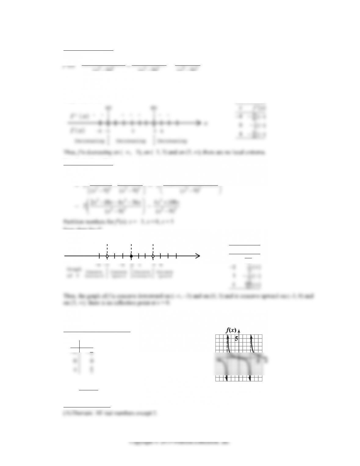
Step 4. Sketch the graph of f:
()
x
fx
44. f(x) =
2
2
56xx
x
Step 1. Analyze f(x):
(A) Domain: All real numbers except x = 0.
(B) Intercepts: y-intercept: f(x) is not defined at 0.
(C) Asymptotes:
Step 2. Analyze f ꞌ(x):
f ꞌ(x) =
22
4
(2 5) 2 ( 5 6)xx xx x
x
=
323 2
4
2521012
x
xx x x
x
=
2
43
512512xxx
xx
Critical values: x = –12
f(x)
5
–
17()
x
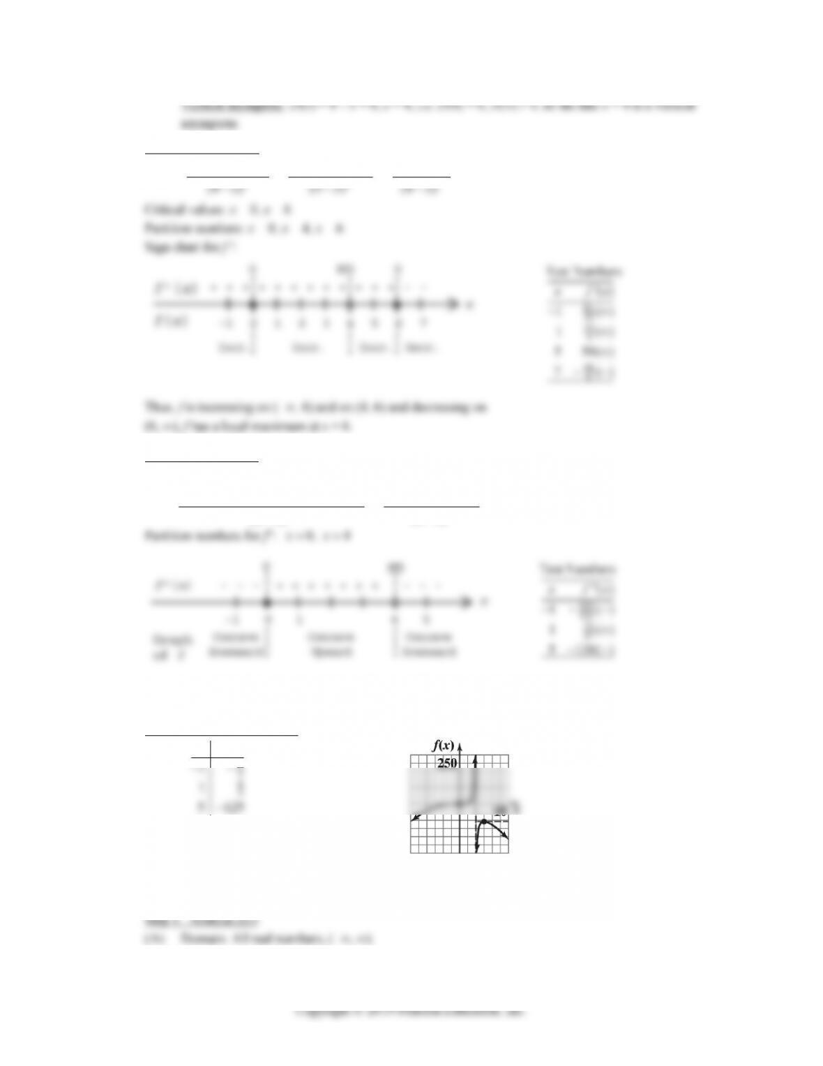
Step 3. Analyze f“(x):
32
EXERCISE 11-4 11-45
5
-4 -2 0 1
21()
x
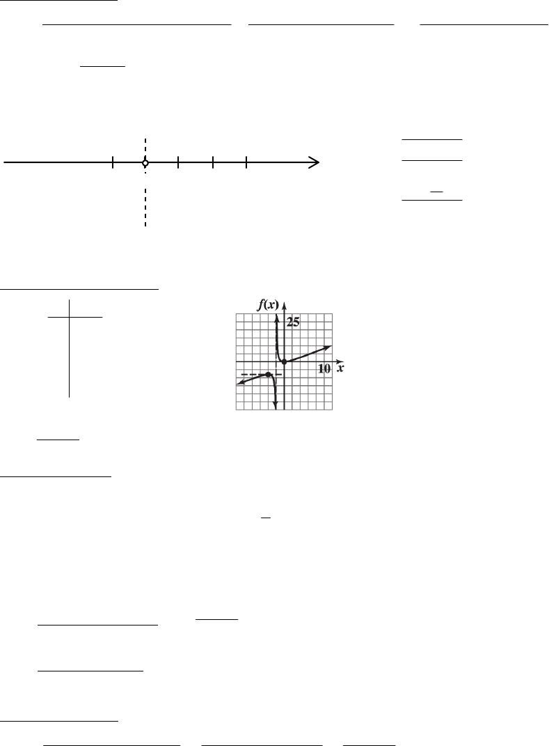
5.
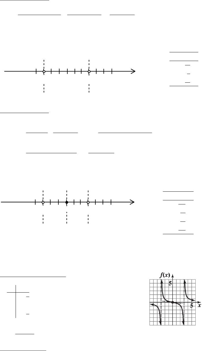
Sketch the graph of f:
15
()
x
fx
46. f(x) =
2
x
x
Step 1. Analyze f(x):
(A) Domain: All real numbers except x = –2.
(B) Intercepts: y-intercept: f(0) = 0
x
x
(C) Asymptotes:
Horizontal asymptote: lim
x
2
2
x
x
= ∞, so there is no horizontal asymptote.
Step 2. Analyze f ꞌ(x):
f ꞌ(x) =
222
222
2(2 ) 4 2 (4 )
(2 ) (2 ) (2 )
x
xx x x x x x
x
xx
Critical values: x = –4, x = 0
x
11-46 CHAPTER 11: GRAPHING AND OPTIMIZATION
Step 3. Analyze f“(x):
2
(4 2 )(2 ) 2(2 ) (4 )
x
xxxx
(4 2 )(2 ) 2 (4 )
x
xxx
22
88 2 8 2
x
xxx
x
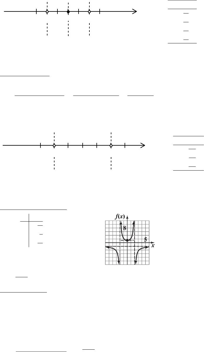
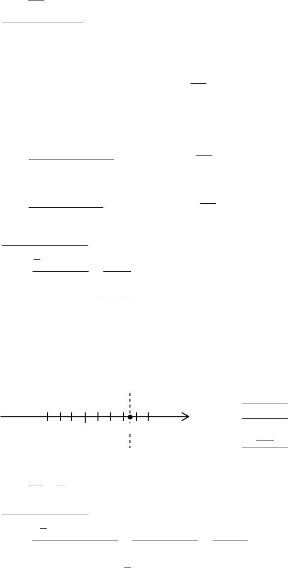
Partition numbers for f“: x = –2
Sign chart for f“:
f“(x)
– – – + + + + +
ND
Test Numbers
“( )
x
fx
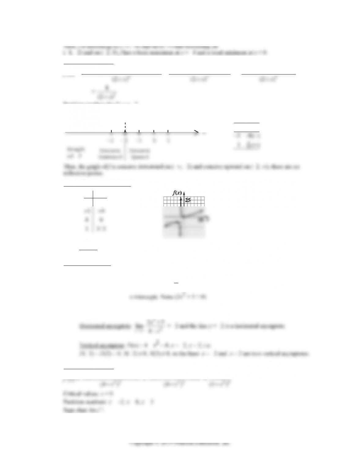
Step 4. Sketch the graph of f:
()
48
x
fx
48. f(x) =
2
2
25
4
x
x
Step 1. Analyze f(x):
(A) Domain: All real numbers except x = –2, x = 2.
(B) Intercepts: y-intercept: f(0) = 5
4
(C) Asymptotes:
x
Step 2. Analyze f ꞌ(x):
22
4(4 ) 2(2 5)
xx xx
33
16 4 4 10
x
xx x
26
x
EXERCISE 11-4 11-47
f‘(x)
– – – – – – + + + + + +
ND 0 ND
Test Numbers
‘( )
x
fx
Step 3. Analyze f“(x):
f“(x) = 26(4 – x2)–2 + 4x(4 – x2)–3(26x)
x
x
f“(x)
x
– – – + + + + + + + – – –
ND
-3 -2 0 2 3
ND Test Numbers
806
125
104
“( )
3()
0()
x
fx
Step 4. Sketch the graph of f:
23
()
x
fx
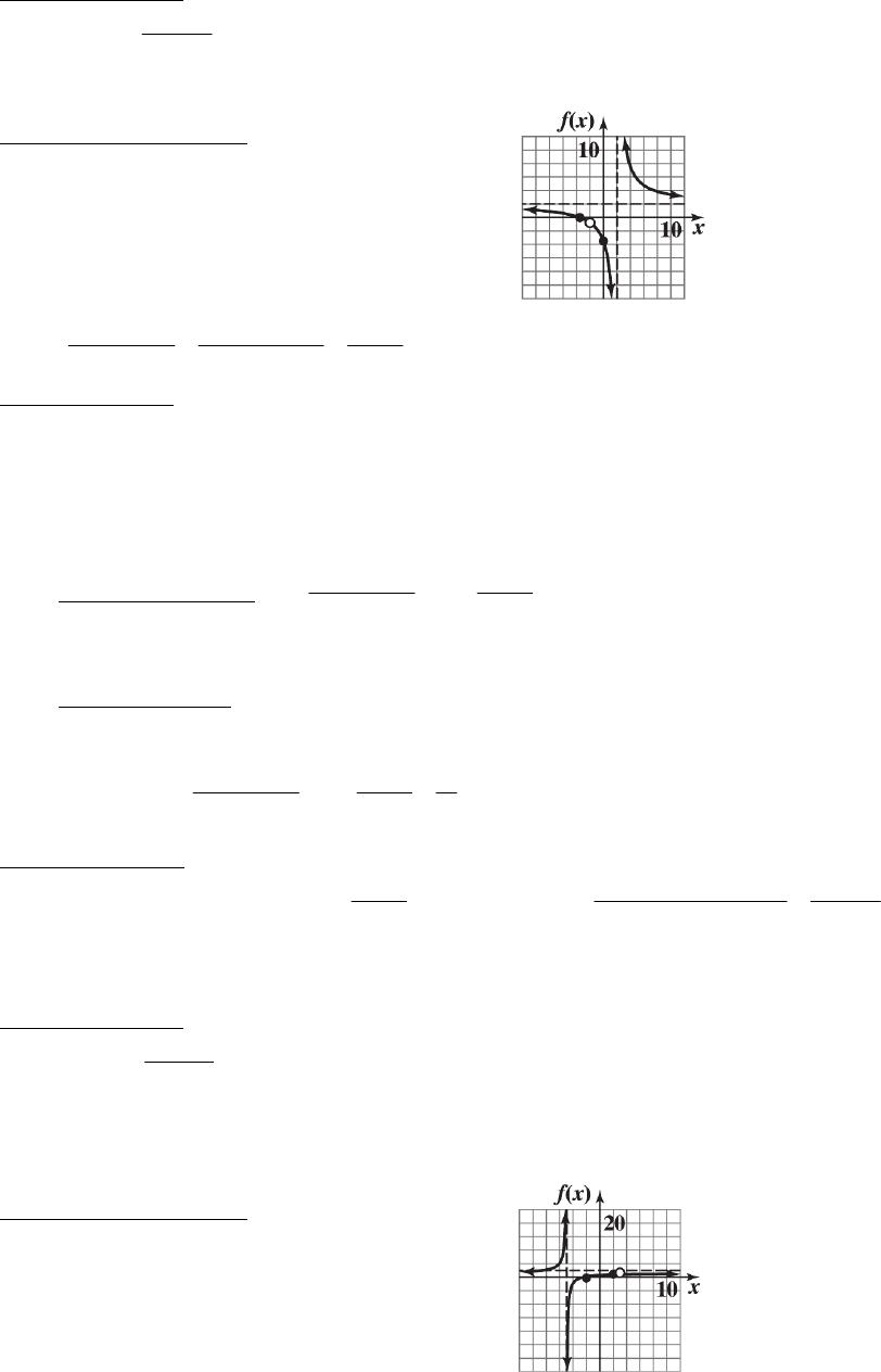
50. f(x) =
3
4
x
x
Step 1. Analyze f(x):
(A) Domain: All real numbers except x = 4.
(B) Intercepts: y-intercept: f(0) = 0
x
11-48 CHAPTER 11: GRAPHING AND OPTIMIZATION
Step 2. Analyze f ꞌ(x):
f ꞌ(x) =
23
2
3(4 )
x
xx
233
2
12 3
x
xx
2
2
2(6 )
x
x
x
Step 3. Analyze f“(x):
f“(x) = (24x – 6x2)(4 – x)–2 + 2(4 – x)–3(12x2 – 2x3)
=
223
3
(246)(4)2(12 2)
(4 )
x
xx xx
x
=
2
3
2( 12 48)
(4 )
xx x
x
x
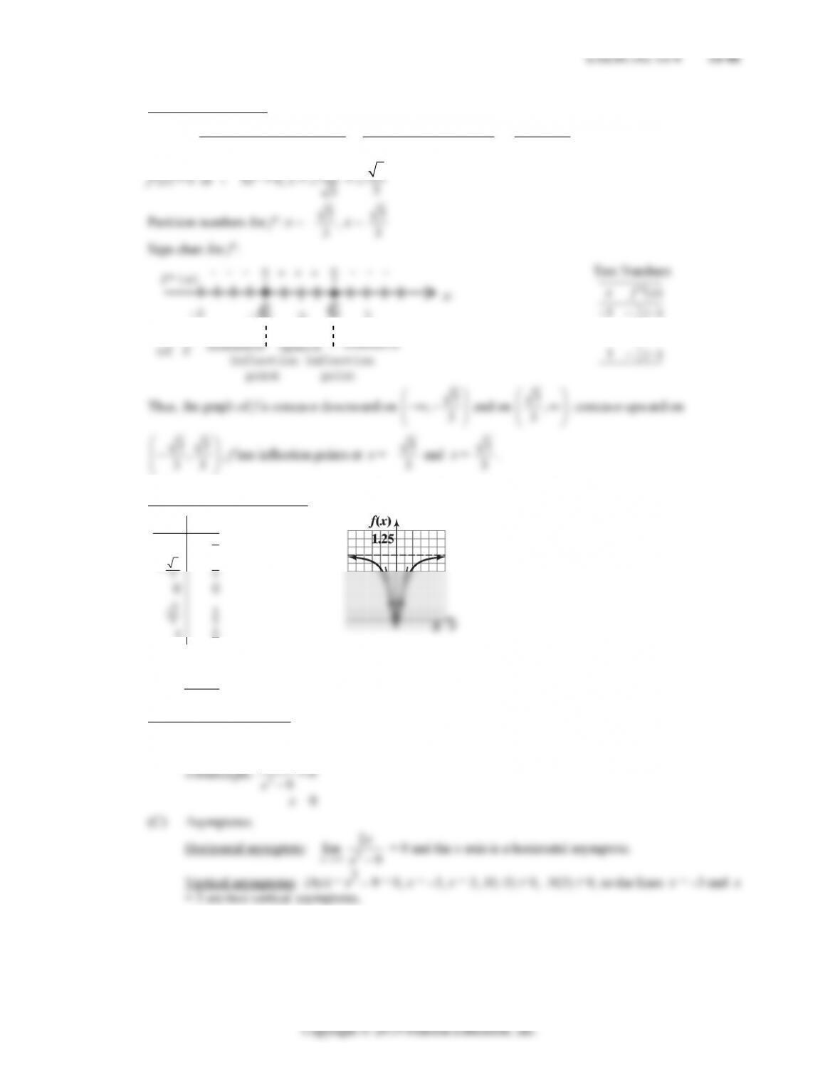
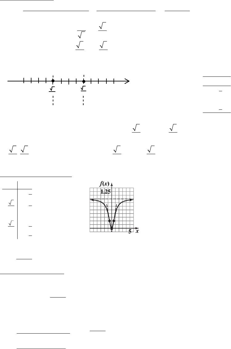
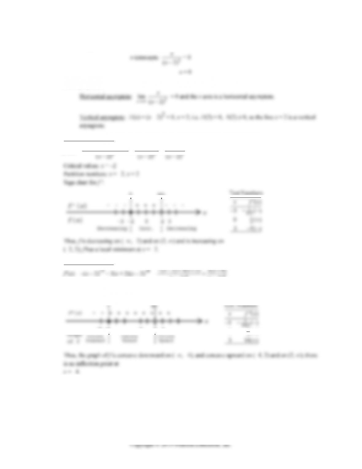
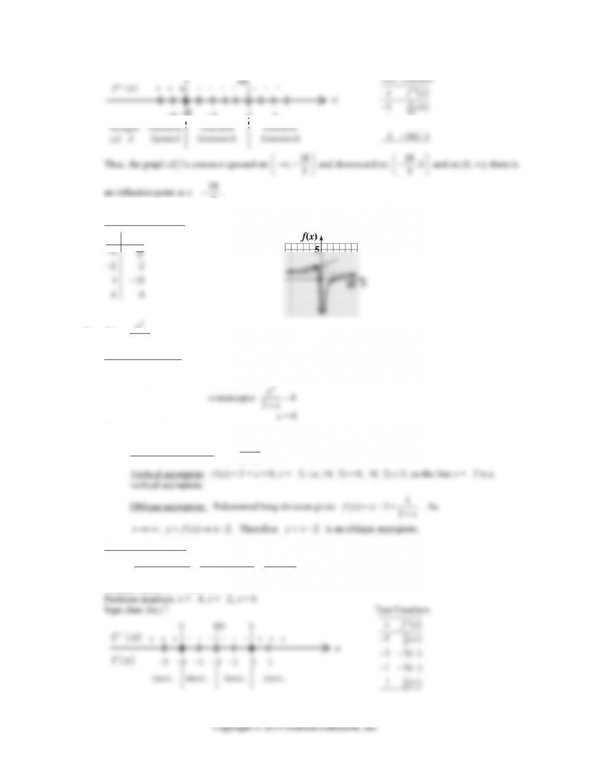
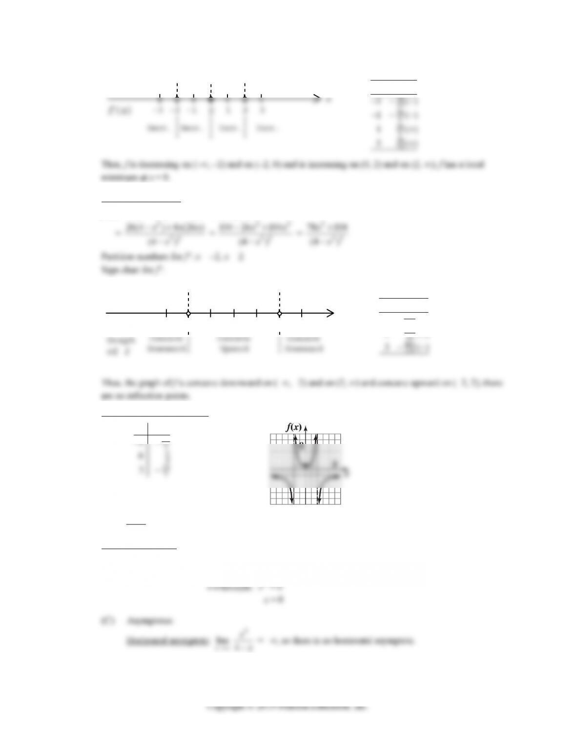
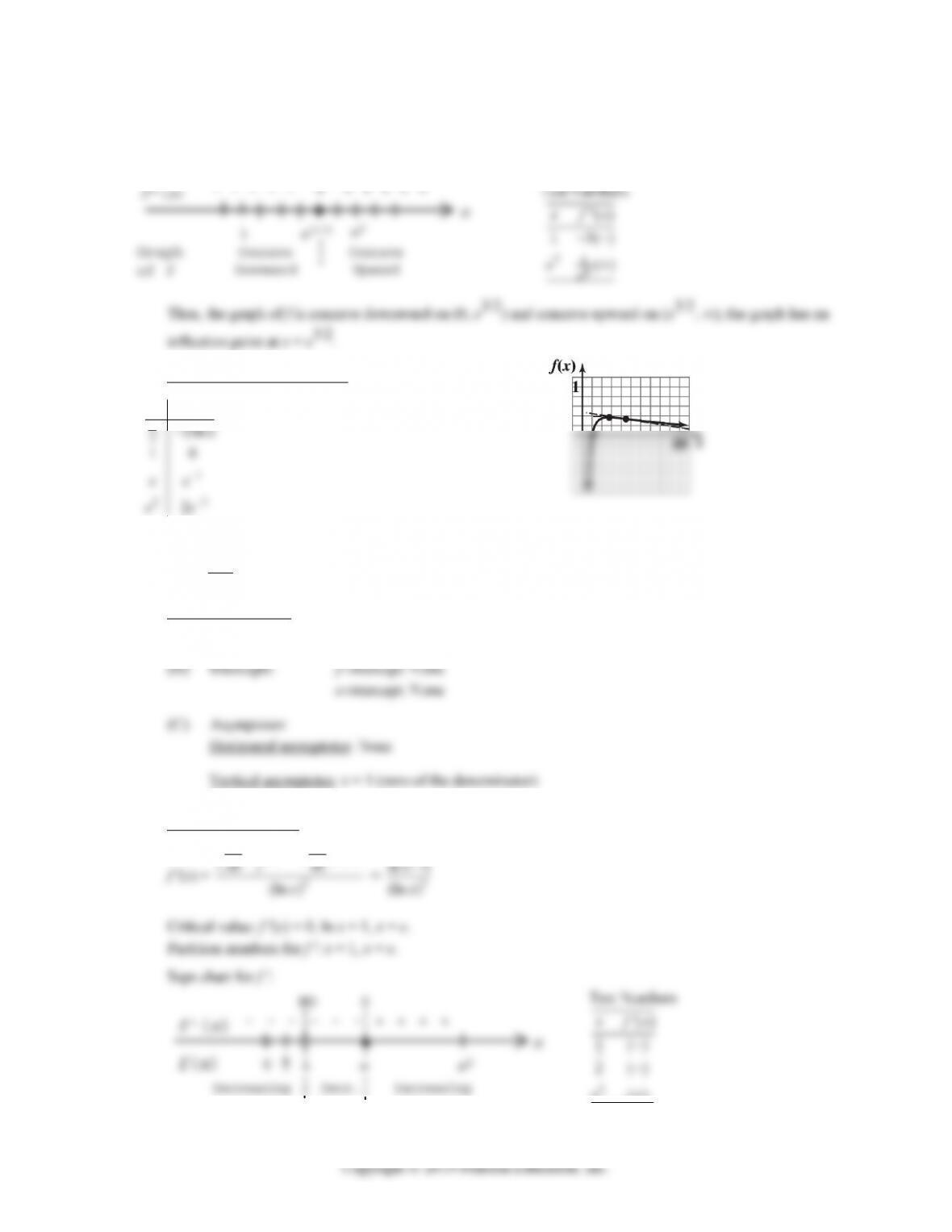
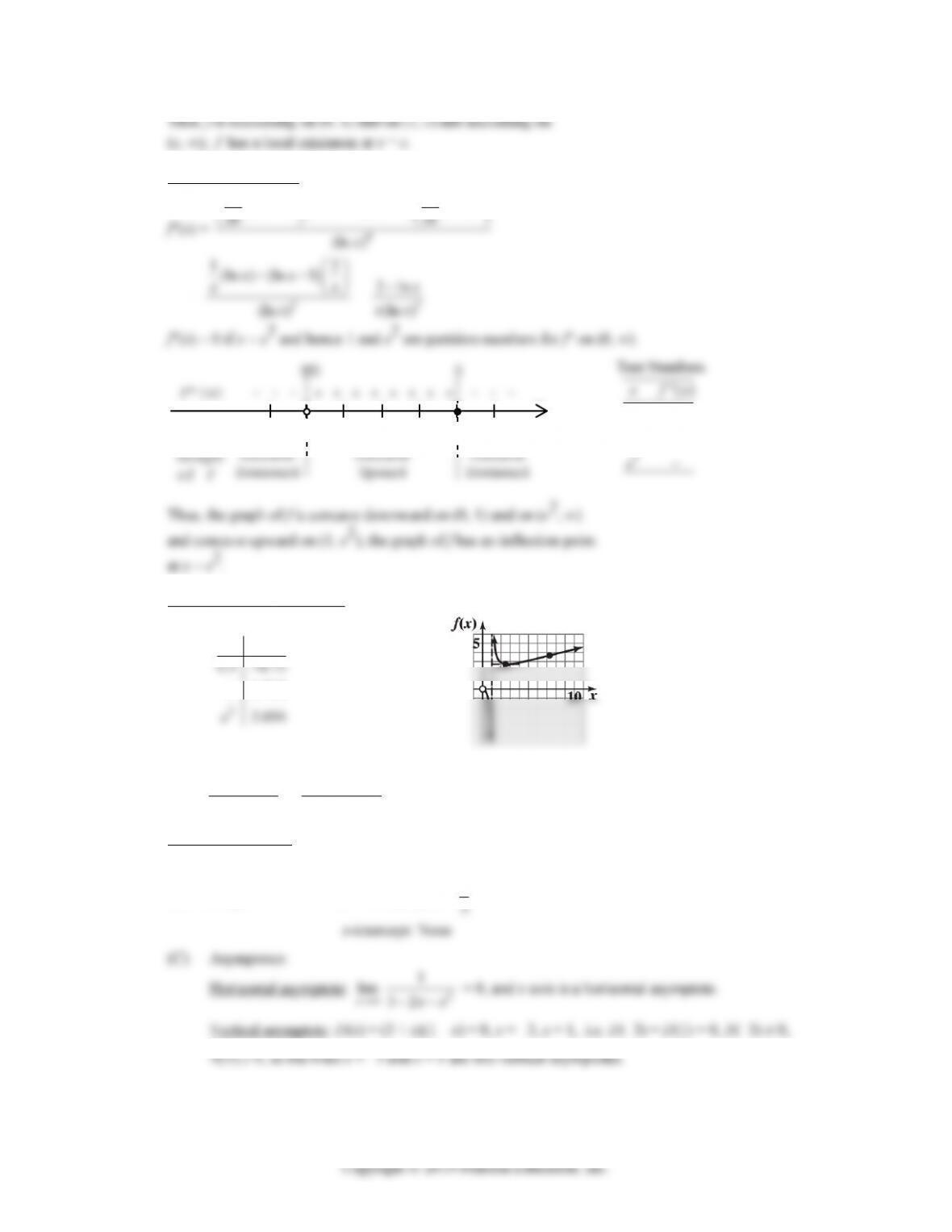
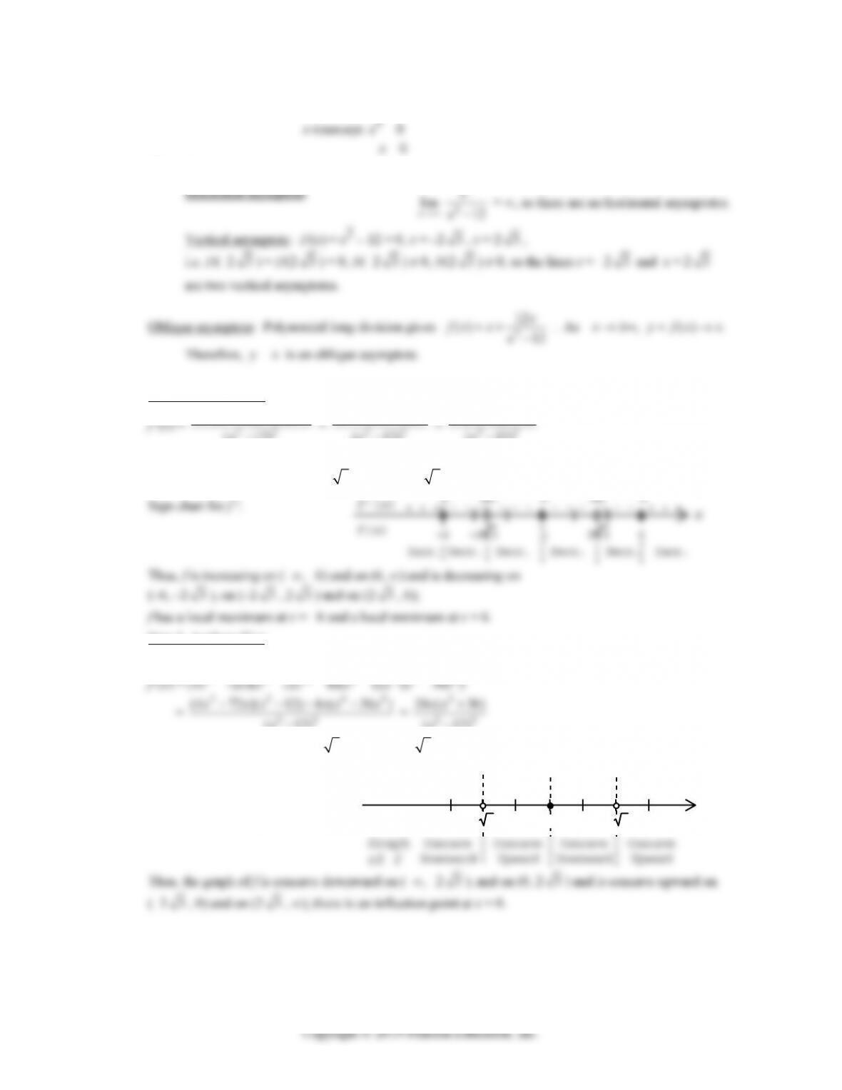
Thus, the graph of f is concave downward on (–∞, 0) and on (4, ∞) and concave upward on (0, 4); there is
an inflection point at x = 0.
Step 4. Sketch the graph of f:
1
()
x
fx
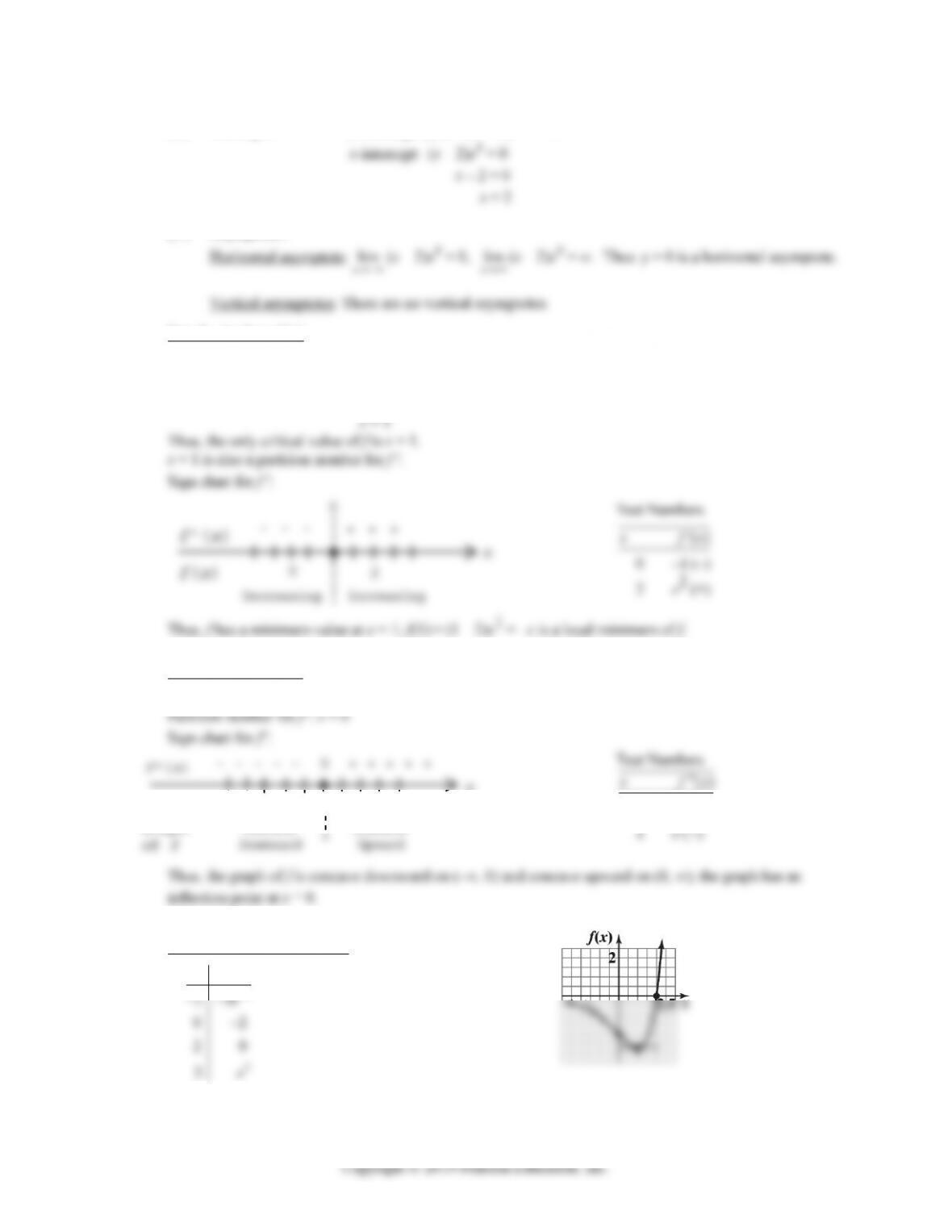
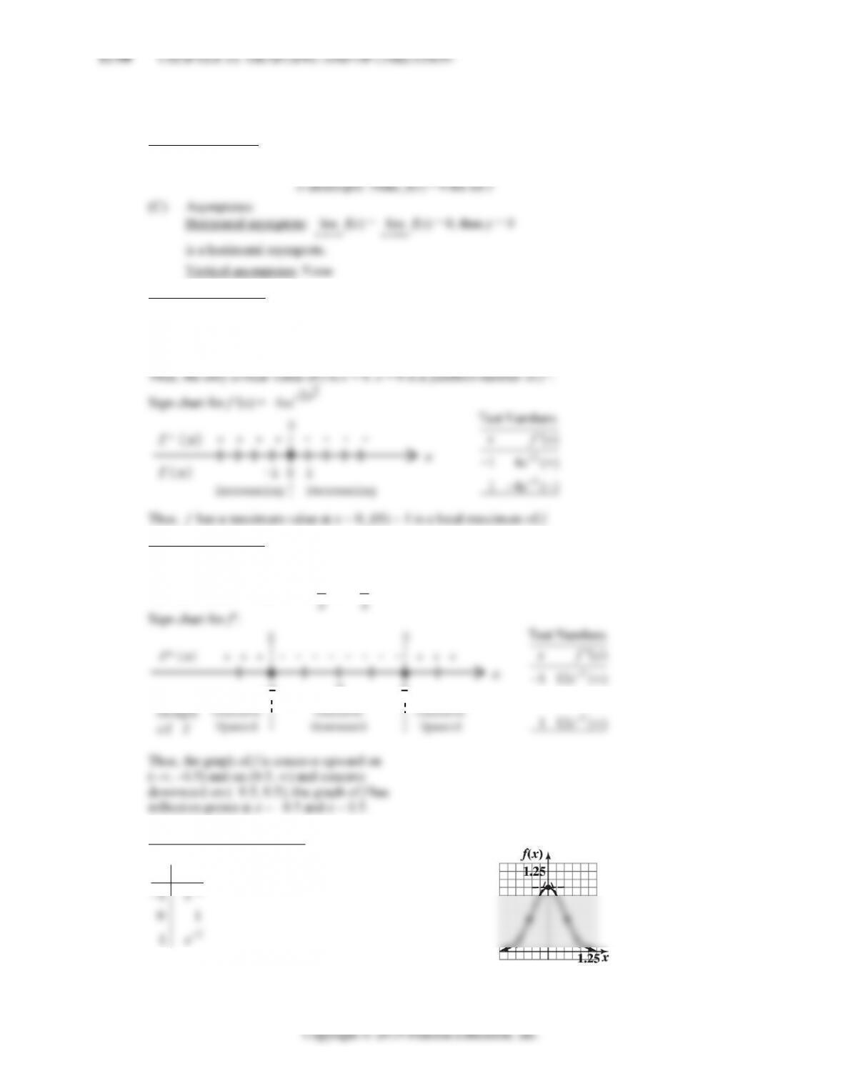
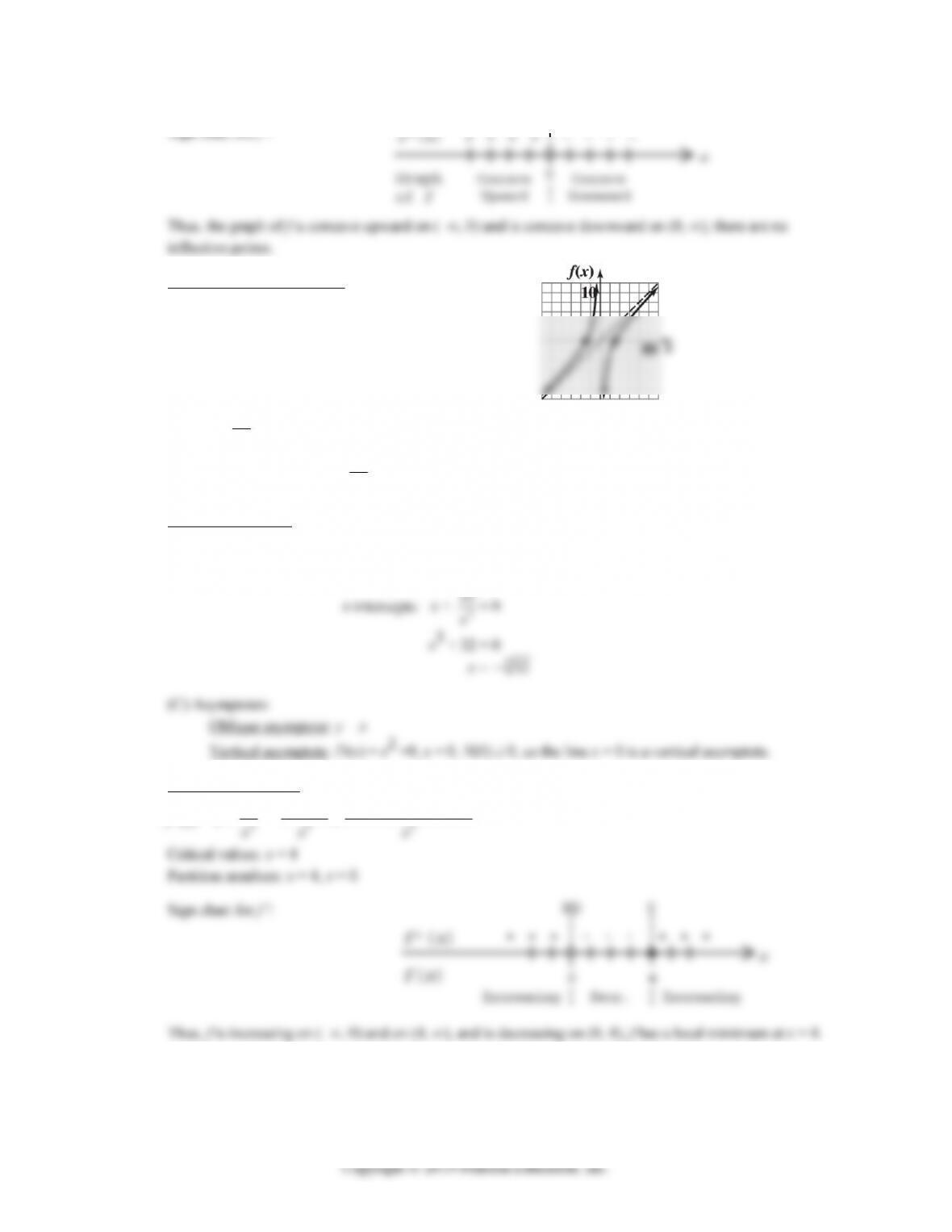
52. f(x) = (x – 2)ex
EXERCISE 11-4 11-49
(B) Intercepts: y-intercept: f(0) = (0 – 2)e0 = –2
(C) Asymptotes:
Step 2. Analyze f ꞌ(x):
f ꞌ(x) = ex + (x – 2)ex = (x – 1)ex
Critical values: f ꞌ(x) = (x – 1)ex = 0
x – 1 = 0
x
Step 3. Analyze f“(x):
f“(x) = ex + (x – 1)ex = xex
x
Graph
Concave
-1 1
Concave
0
–1 –e–1 (–)
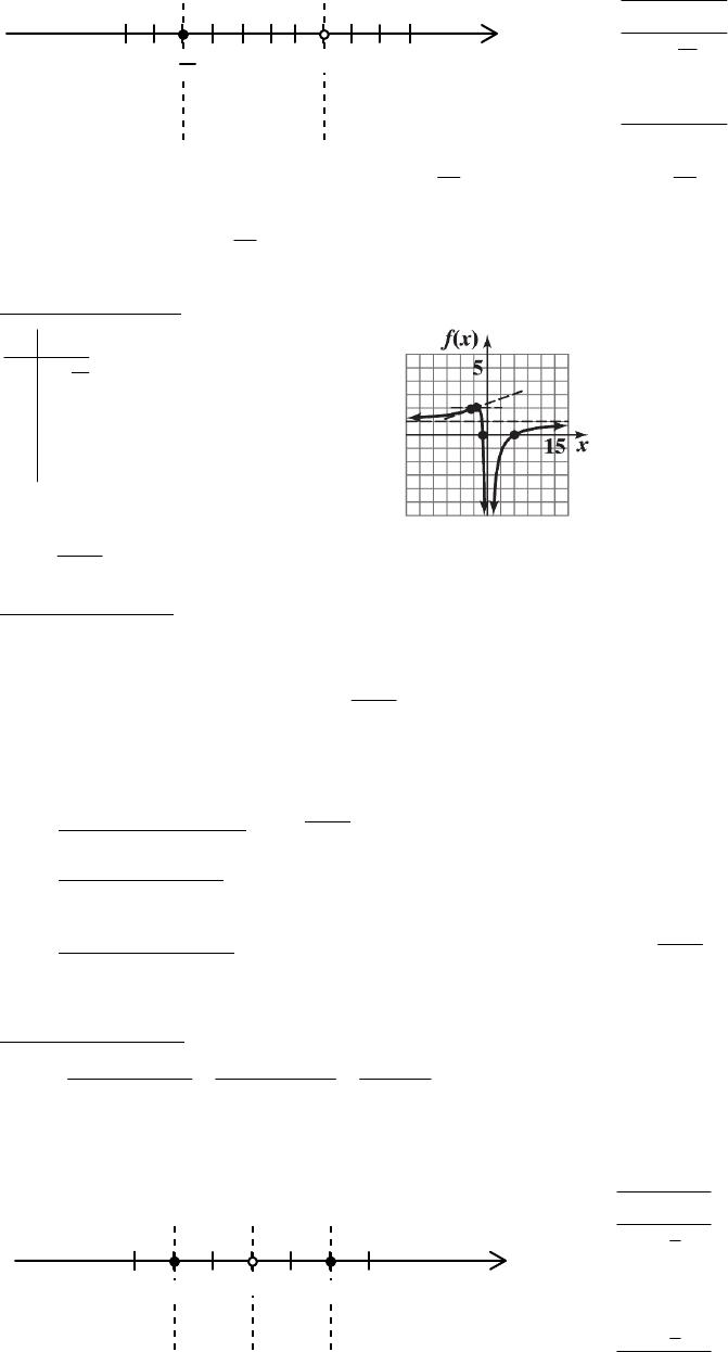
Step 4. Sketch the graph of f:
1
()
x
fx
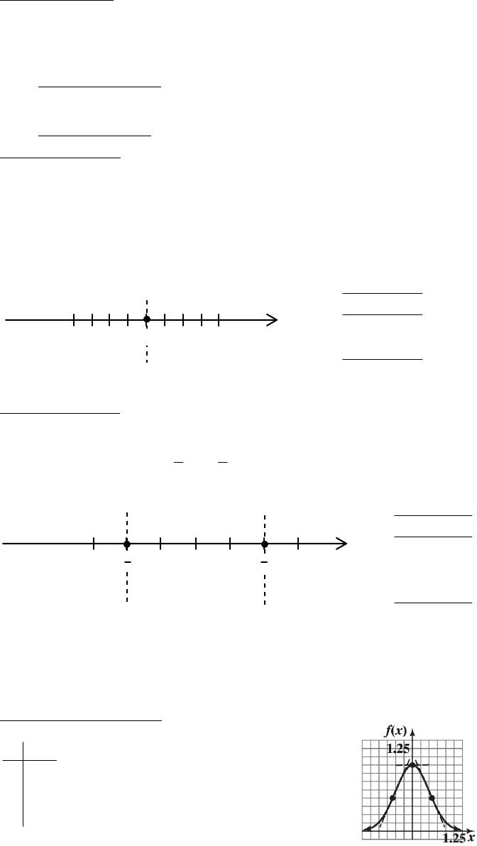
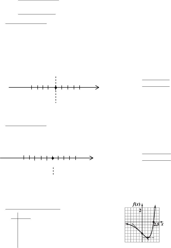
54. f(x) = e–2x2
Step 1. Analyze f(x):
(A) Domain: All real numbers, (–∞, ∞).
(B) Intercepts: y-intercept: 1
Step 2. Analyze f ꞌ(x):
f ꞌ(x) = –4xe–2x2
Critical values: f ꞌ(x) = –4xe–2x2 = 0
x = 0
Step 3. Analyze f“(x):
f“(x) = –4e–2x2 – 4x(–4x)e–2x2 = (16x2 – 4)e–2x2
Partition numbers for f“: x = –1
–1
201
2
04()
x
Step 4. Sketch the graph of f:
2
()
x
fx
56. f(x) = ln
x
x
.
Step 1. Analyze f(x):
(A) Domain: All positive real numbers, (0, ∞).
(B) Intercepts: y-intercept: Does not exist;
0 is not in the domain of f.
x
x
x
x
x
x
Step 2. Analyze f ꞌ(x):
f ꞌ(x) = 2
1() (1)ln
x
x
x
x
= 2
1ln
x
x
1ln
x
= 0
Step 3. Analyze f“(x):
2
1()2(1ln)
11-52 CHAPTER 11: GRAPHING AND OPTIMIZATION
Thus, x = e3/2 is a partition number for f“.
Sign chart for f“:
x
Step 4. Sketch the graph of f:
1
()
x
fx
58. f(x) = ln
x
x
Step 1. Analyze f(x):
(A) Domain: All positive real numbers, except x = 1.
Step 2. Analyze f ꞌ(x):
ln (ln )
dd
x
xx x
x
x
()
e
EXERCISE 11-4 11-53
Step 3. Analyze f“(x):
22
(ln 1) (ln ) (ln 1) (ln )
dd
xxx x
x
e2
1
0.5
e
Step 4. Sketch the graph of f:
()
2.718
x
fx
e
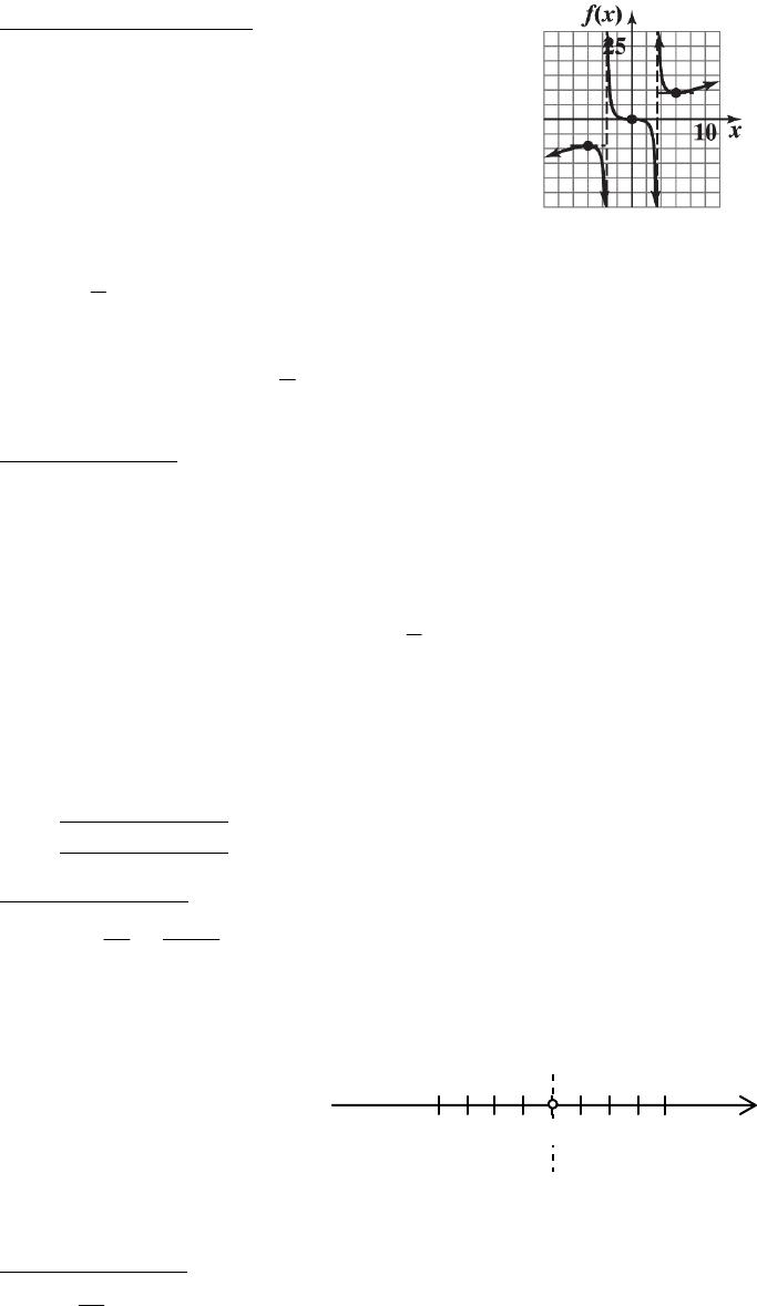
60. f(x) = 2
1
32
x
x = 1
(3 )(1 )
x
x
Step 1. Analyze f(x):
(A) Domain: All real numbers except x = –3, x = 1.
(B) Intercepts: y-intercept: f(0) = 1
11-54 CHAPTER 11: GRAPHING AND OPTIMIZATION
Step 2. Analyze f ꞌ(x):
f ꞌ(x) = 22
22
(3 2 )
x
xx
= 22
2( 1)
(3 2 )
x
xx
Critical values: x = –1
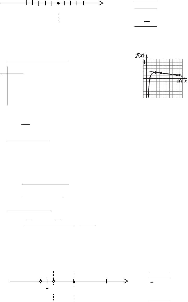
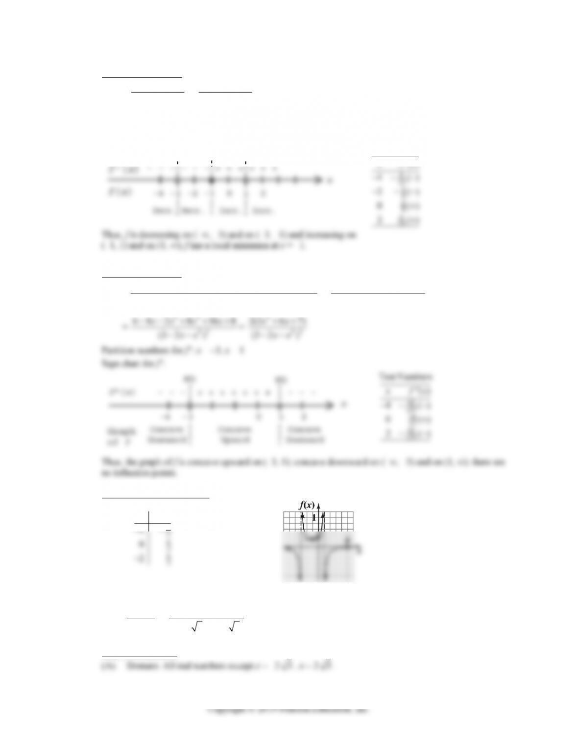
Partition numbers: x = –3, x = –1, x = 1
Sign chart for f ꞌ:
ND 0 ND
Test Numbers
‘( )
x
fx
Step 3. Analyze f“(x):
f“(x) =
22 2
24
2(3 2 ) 2(3 2 )( 2 2 )[2( 1)]
(3 2 )
xx xx x x
xx
=
22
23
2(3 2 ) 8( 1)
(3 2 )
xx x
xx
x
Step 4. Sketch the graph of f:
1
()
x
fx
62. f(x) =
3
212
x
x =
3
23 23
x
xx
Step 1. Analyze f(x):
EXERCISE 11-4 11-55
(B) Intercepts: y-intercept: f(0) = 0
(C) Asymptotes:
3
x
Step 2. Analyze f ꞌ(x):
22 3
3( 12)2()
( 12)
x
xxx
x
=
424
3362
( 12)
x
xx
x
=
2
(6)(6)
(12)
xx x
x
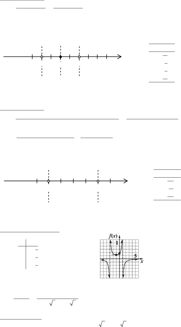
Critical values: x = –6, x = 0, x = 6
Partition numbers: x = –6, x = –23, x = 0, x = 2 3, x = 6
Step 3. Analyze f“(x):
f ꞌ(x) = (x4 – 36x2)(x2 – 12)–2
(12)
x
x
=
( 12)
x
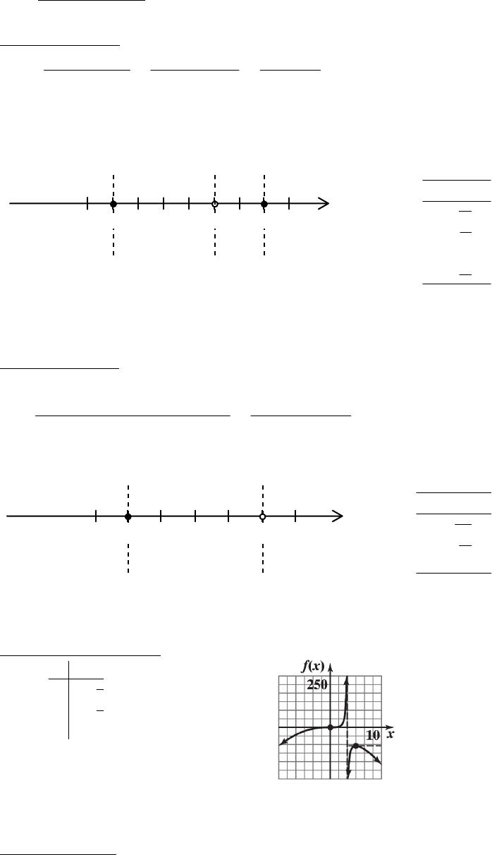
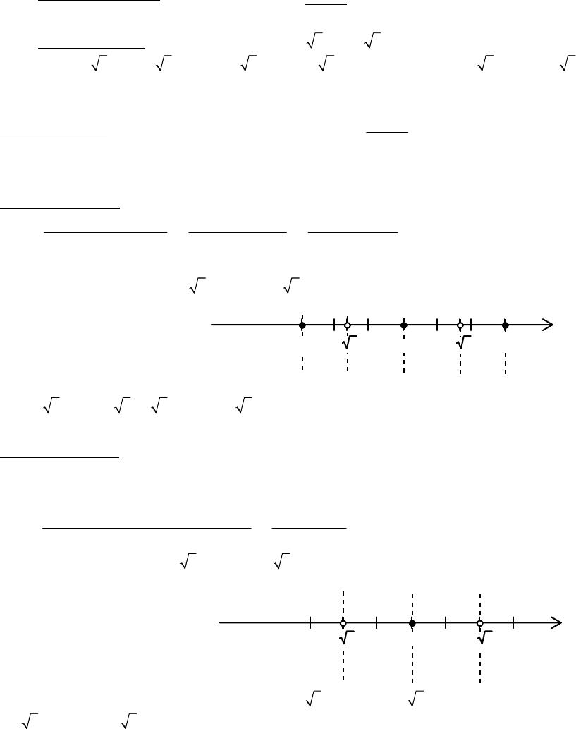
Partition numbers for f“: x = –23, x = 0, x = 2 3
Sign chart for f“:
f“(x)
x
– – – + + + + – – – – + + +
0
ND
-2 3 230
ND
Step 4. Sketch the graph of f:
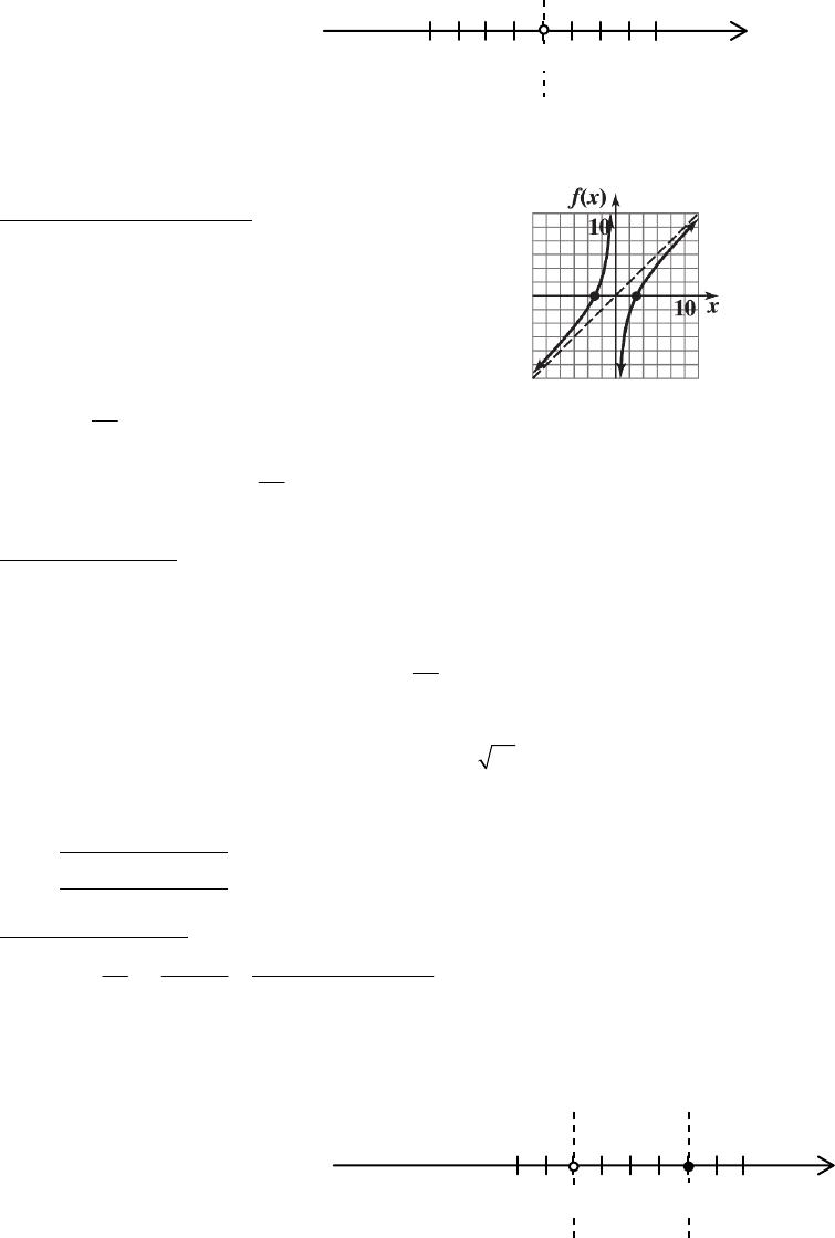
64. f(x) = x – 9
x
For |x| very large, 9
()
f
xx x
x
. Thus, the line y = x is an oblique asymptote.
Step 1. Analyze f(x):
(A) Domain: All real numbers except 0.
(B) Intercepts: y-intercept: There is no y-intercept since
f is not defined at x = 0.
x
(C) Asymptotes:
Step 2. Analyze f ꞌ(x):
9
x
2
9x
x
Step 3. Analyze f“(x):
x
EXERCISE 11-4 11-57
Sign chart for f“: + + + + – – – –
ND
Step 4. Sketch the graph of f:
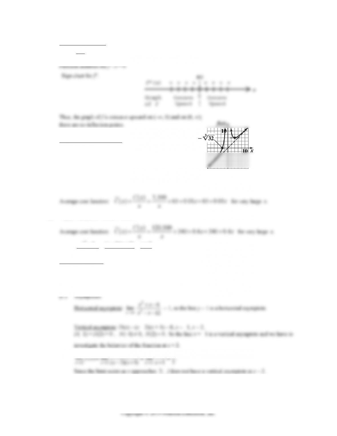
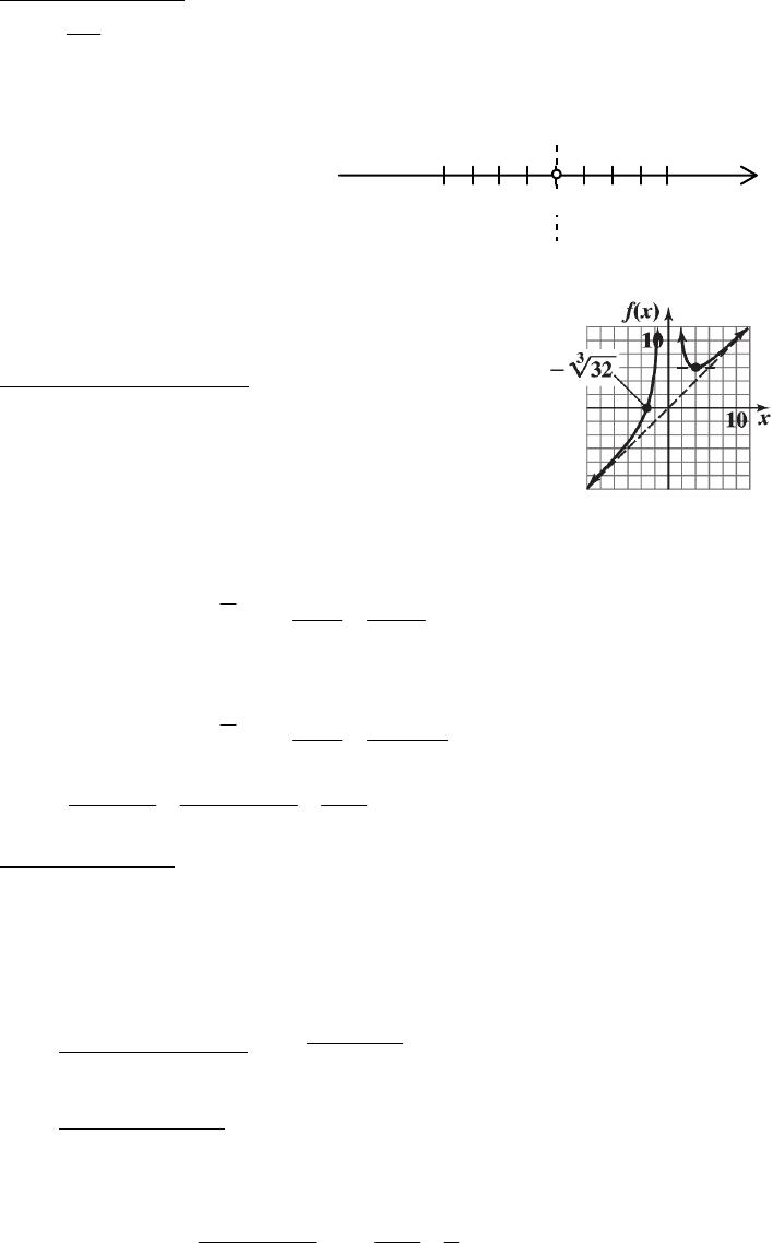
66. f(x) = x + 2
32
x
For |x| very large, f(x) = x +
2
32
x
≈ x. Thus, the line y = x is an oblique asymptote.
Step 1. Analyze f(x):
(A) Domain: All real numbers except 0.
(B) Intercepts: y-intercept: No y-intercept since f is not defined at 0.
x
Step 2. Analyze f ꞌ(x):
f ꞌ(x) = 1 –
64
x
=
32
64 ( 4)( 4 16)xxxx
11-58 CHAPTER 11: GRAPHING AND OPTIMIZATION
Step 3. Analyze f“(x):
f“(x) = 4
192
x
Step 4. Sketch the graph of f:
68. 2
() 7,500 65 0.01 .Cx x x
70. 2
( ) 120,000 340 0.4 .Cx x x
72.
2
2
4(2)(2) 2
() , 2
(2)(1) 1
2
xxxx
fx x
xx x
xx
Step 1. Analyze f(x):
(A) Domain: All real numbers except x = –1, x = 2.
(B) Intercepts: y-intercept: f(0) = 2
x-intercept: x = –2
(2)(2) 24
xx x
Step 2. Analyze f ꞌ(x):
( 1)(1) ( 2)(1) 1
xx
Step 3. Analyze f“(x):
(1)
x
Partition numbers for ”
Sign chart for f“:
Step 4. Sketch the graph of f:
74.
2
22
32(2)(1) 1
() , 2.
2
44 (2)
xx x x x
fx x
x
xx x
Step 1. Analyze f(x):
(A) Domain: All real numbers except x = 2.
(B) Intercepts: y-intercept: f(0) = 1
Step 2. Analyze f ꞌ(x):
We can express f(x) for x ≠ 2 as f(x) = 1
x

11-60 CHAPTER 11: GRAPHING AND OPTIMIZATION
Step 3. Analyze f“(x):
Step 4. Sketch the graph of f:
76.
2
2
2 15(25)(3)25
() , 3.
(5)(3) 5
215
xx x x x
fx x
xx x
xx
Step 1. Analyze f(x):
(A) Domain: All real numbers except x = –5, x = 3.
(B) Intercepts: y-intercept: f(0) = 1
(C) Asymptotes:
Step 2. Analyze f ꞌ(x):
x
(5)(2)(25)(1) 5
xx
Step 3. Analyze f“(x):
10
Step 4. Sketch the graph of f: