
EXERCISE 11-2 11-21
80. f(x) = x4 + 2x3 – 5x2 – 4x + 4
Step 1. Analyze f(x):
(A) Domain: all real numbers
(B) Intercepts: y-intercept: f(0) = 4
Step 2. Analyze f ꞌ(x): f ꞌ(x) = 4x3 + 6x2 – 10x – 4
Critical values: x = –2.38, –0.35, 1.22
Step 3. Analyze
f
(x): f“(x) = 12x2 + 12x – 10
82. f(x) = – x4 + x3 + x2 + 6
Step 1. Analyze f(x):
(A) Domain: all real numbers
(B) Intercepts: y-intercept: f(0) = 6
f
84. The graph of the PPI is concave downward.
86. The graph of ‘( )Cx is positive and increasing. Since the marginal costs are increasing, the production
88. P(x) = R(x) – C(x)
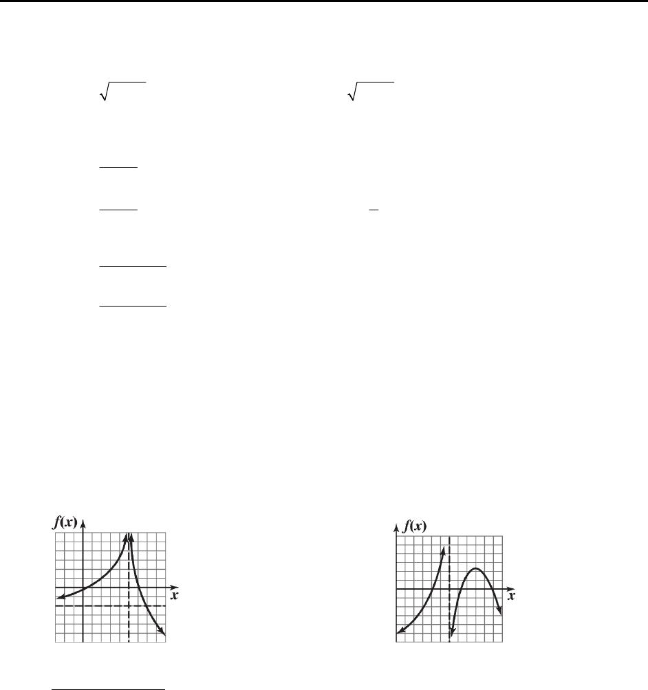
= 1,296x – 0.12x3 – (830 + 396x) = 1,296x – 0.12x3 – 830 – 396x = 900x – 0.12x3 – 830
11-22 CHAPTER 11: GRAPHING AND OPTIMIZATION
90. p = 8 – 2 ln x, 5 ≤ x ≤ 50
The revenue function is:
R(x) = xp(x) = x(8 – 2 ln x) = 8x – 2x ln x, 5 ≤ x ≤ 50.
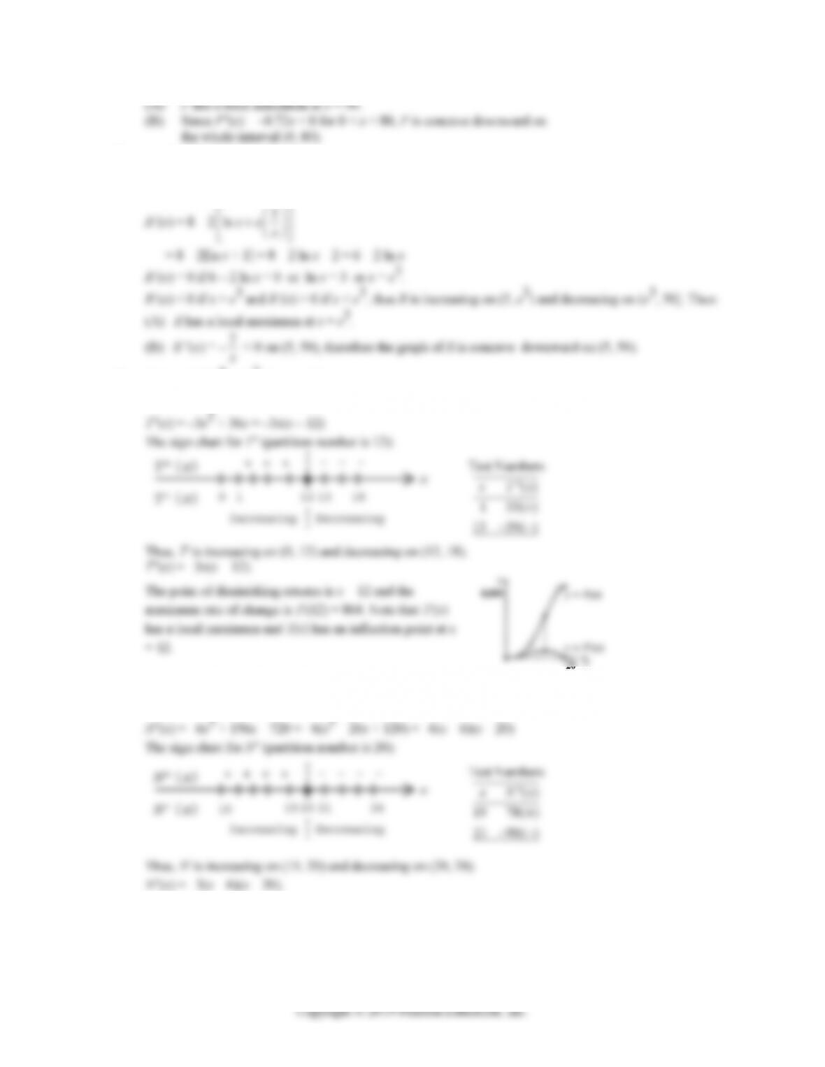
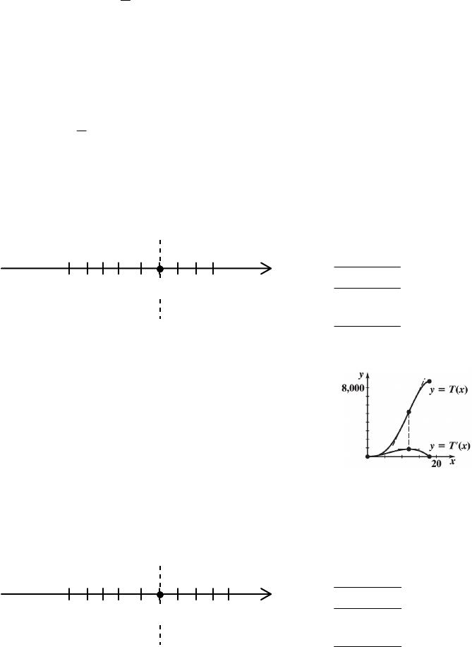
92. T(x) = –0.25x4 + 6x3, 0 ≤ x ≤ 18
T‘(x) = –x3 + 18x2 = –x2(x – 18)
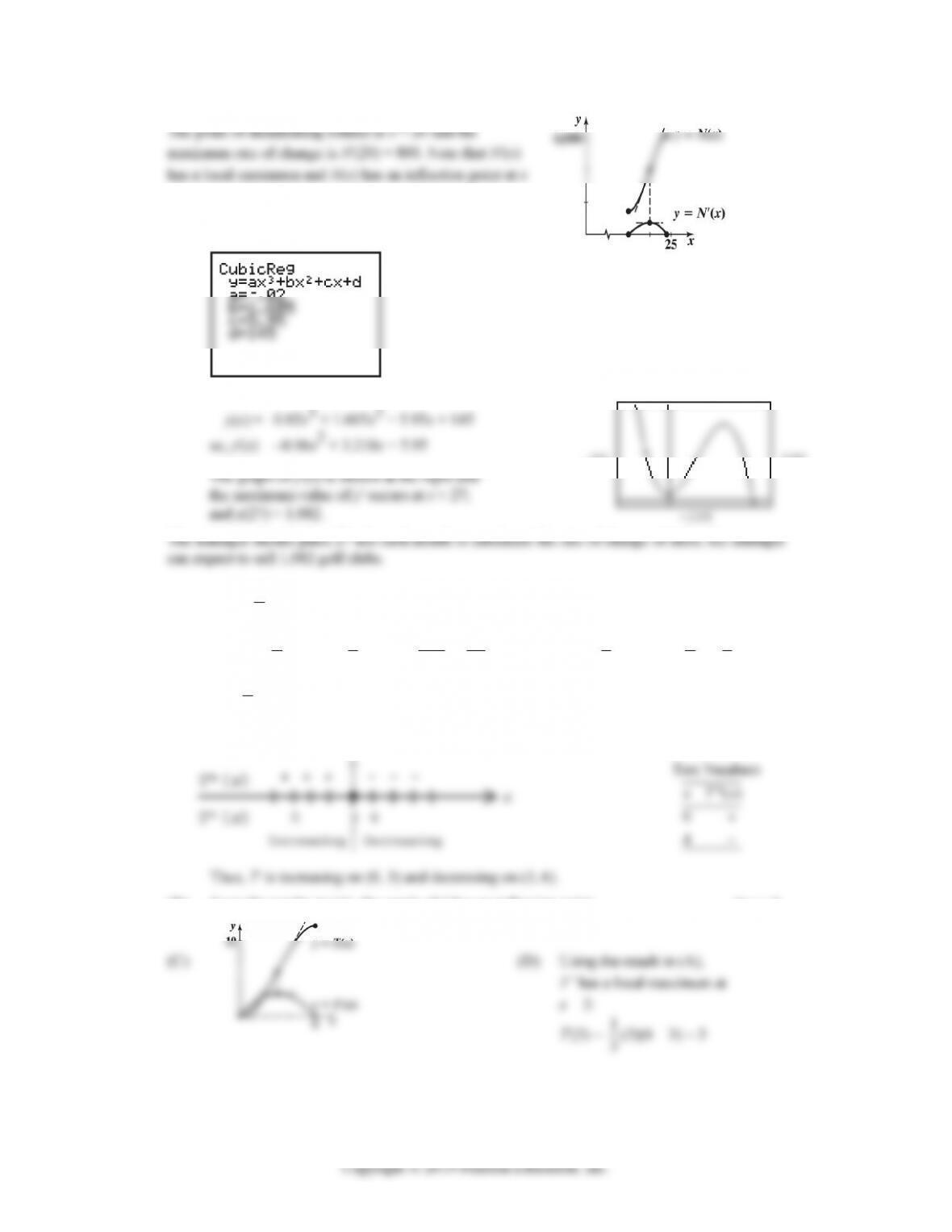
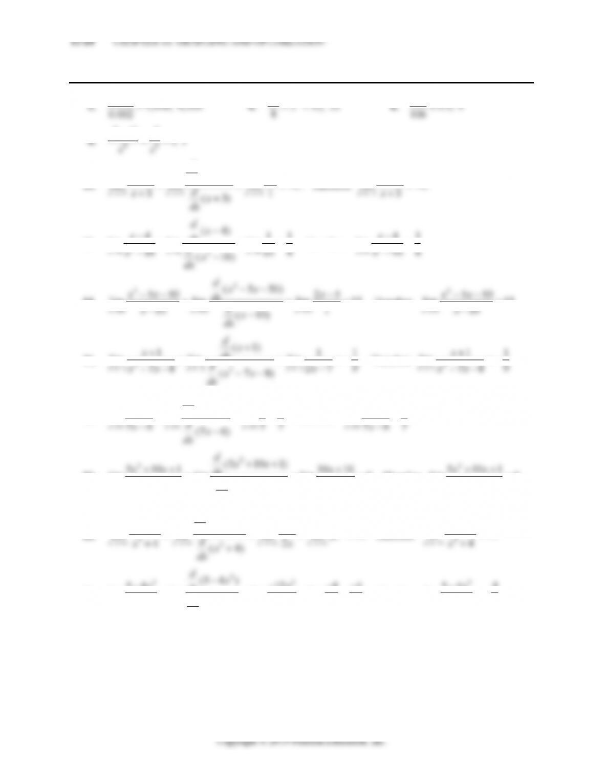
94. N(x) = –0.5x4 + 26x3 – 360x2 + 20,000, 15 ≤ x ≤ 24
N‘(x) = –2x3 + 78x2 – 720x
EXERCISE 11-2 11-23
= 20.
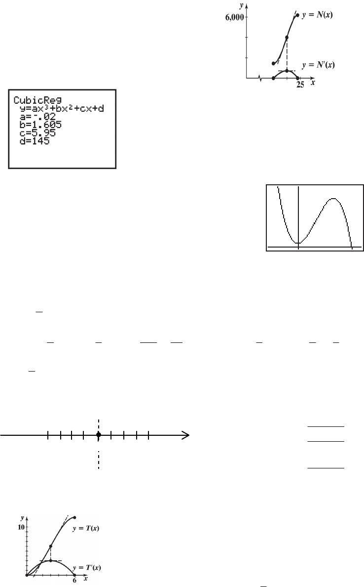
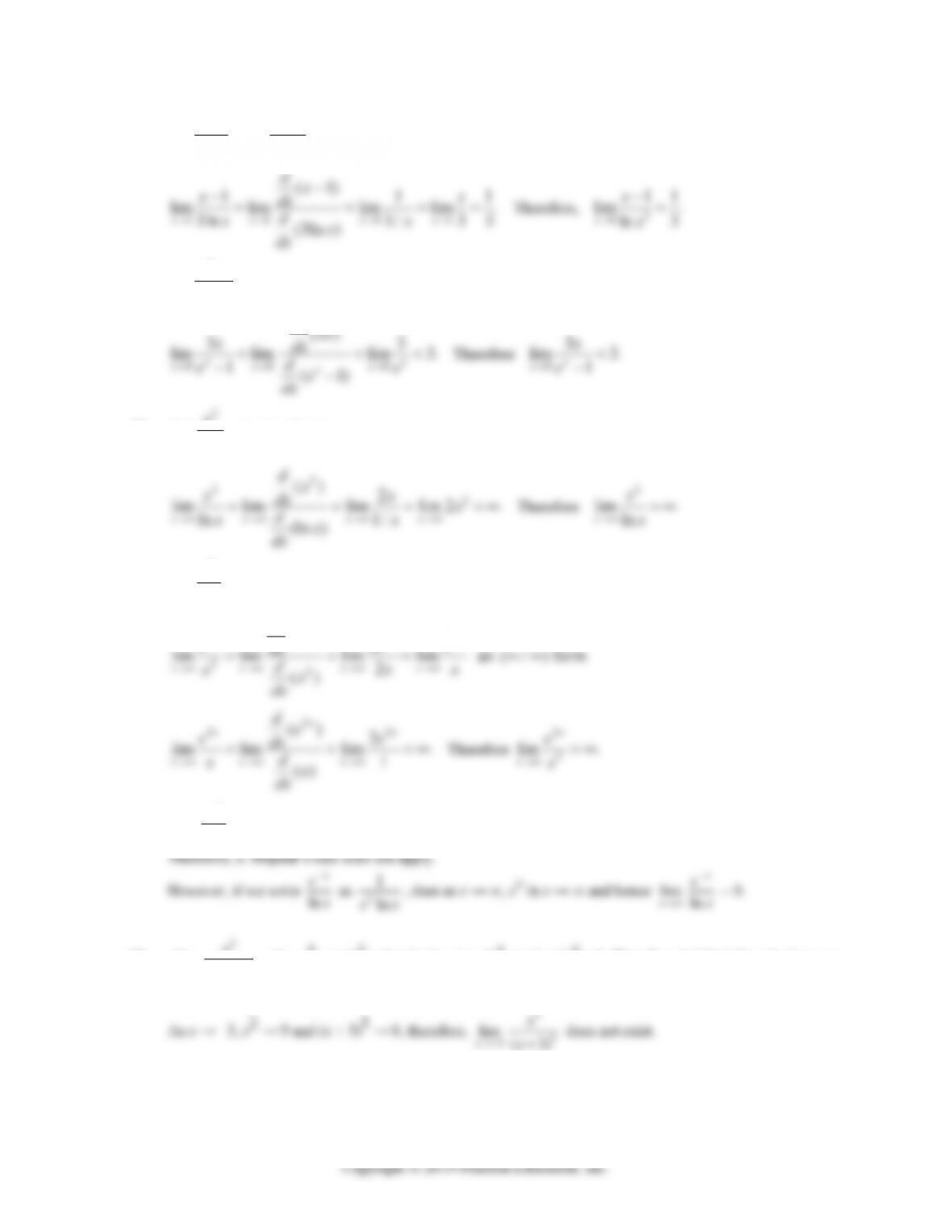
96. (A)
(B) From part (A),
-50
100
2500
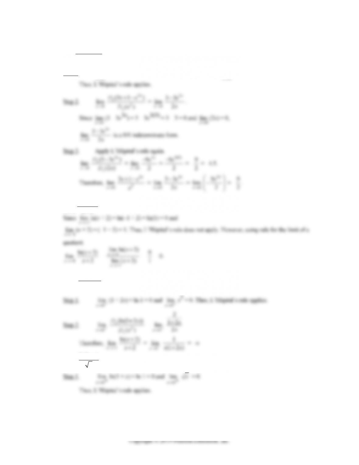
98. T(x) = x219
x
, 0 ≤ x ≤ 6
‘( )Tx = 2x19
x
+ x21
9
= 2x –
2
2
9
x
–
2
9
x
= 2x – 1
3x2 = x23
x
= 1
3x(6 – x)
T“(x) = 2 – 2
3x = 0, x = 3
(A) The sign chart for T” (partition number is 3) is:
x
(B) From the results in (A), the graph of T has an inflection point at x = 3.

EXERCISE 11–3
8
5
2232;32
82 8
51; 1
ee
10.
2
2
(9)
92
lim lim lim 6
dx
xx
dx
. Therefore
2
9
lim 6.
x
12. 2
411
lim lim lim .
xdx
Therefore, 2
41
lim .
x
14.
lim lim lim 15.
dx
Therefore
lim 15.
16. 2
lim lim lim .
Therefore 2
lim .
18.
(6 7)
67 66
lim lim lim .
dx
xdx
Therefore 676
lim .
x
20.
42 3
42
lim lim lim 0.
142
(1)
xx x
dx
d
xx x x
xx
dx
Therefore
42
lim 0.
1
x
x
x
22.
4
43
2
( 16)
16 4
lim lim lim lim 2 .
dx
xx
dx x
Therefore
4
16
lim .
x
x
24.
32
3
54 12 4 4
lim lim lim lim .
77
17 21
(1 7 )
xx xx
xx
dx
d
xx
x
dx
Therefore
3
54 4
lim .
7
17
x
x
x

EXERCISE 11-3 11-25
26. 3
11
11
lim lim 3ln
ln
xx
xx
x
x
(0/0 form)
28. 0
3
lim 1
x
x
x
e
(0/0 form)
dx
30.
lim ln
x
x
x
( /
form)
32.
2
2
lim
x
x
e
x
( / form)
2
222
() 2
x
xxx
de
eee
34. lim
x ln
x
e
x
; lim
x e-x = 0 and lim
x ln x = ∞.
x
x
x
36. 3
lim
x
5
(3)
x
x; 3
lim
x x2 = (–3)2 = 9 and 3
lim
x (x + 3)5 = (–3 + 3)5 = 0. Therefore, L’Hôpital’s rule does not
apply.

11-26 CHAPTER 11: GRAPHING AND OPTIMIZATION
38.
0
lim
x
3
2
31
x
x
e
x
Step 1.
0
lim
x(3x + 1 – e3x) = 3(0) + 1 – e3(0) = 1 – 1 = 0 and
0
lim
xx2 = 0.
x
x
x
x
x
x
x
x
x
x
x
40. 1
lim
x
ln( 2)
2
x
x
42.
0
lim
x2
ln(1 2 )
x
x
x
x
x
44.
0
lim
x
ln(1 )
x
x

EXERCISE 11-3 11-27
x
x
x
x
x
x
46. 1
lim
x
32
3
231
32
xx
xx
Step 1. 1
lim
32
(2 3 1)
x
Dx x
2
66
x
x
x
x
x
48. 3
lim
x
32
2
33
69
xxx
xx
50.
1
lim
x
32
32
1
331
xxx
x
xx
x

11-28 CHAPTER 11: GRAPHING AND OPTIMIZATION
52. lim
x
2
2
49
58
x
x
x
Step 1. lim
x (4x2 + 9x) = ∞ and lim
x (5x2 + 8) = ∞.
x
x
x
54. lim
x
3
3
x
e
x
Step 1. lim
x e3x = ∞ and lim
x x3 = ∞. Thus, L’Hôpital’s rule applies.
x
x
x
x
x
x
x
x
x
x
x
x
x
x
x
x
x
56. lim
x 2
1
1
x
e
x
Step 1. lim
x (1 + e-x) = ∞ and lim
x (1 + x2) = ∞.
Step 2. lim
(1 )
x
x
De
x
e
x
=
x
x
x
x
x


EXERCISE 11-3 11-29
58. lim
x
ln(1 2 )
ln(1 )
x
x
e
e
Step 1. lim
x ln(1 + 2e-x) = ln 1 = 0 and lim
x ln(1 + e-x) = ln 1 = 0.
x
x
x
x
x
x
x
x
60. 0
lim
x
22
3
12 2
x
exx
x
Step 1. 0
lim
x(e2x – 1 – 2x – 2x2) = e2(0) – 1 – 2(0) – 2(0)2 = 0 and
Step 2. 0
lim
x
22
3
(122)
()
x
x
x
De x x
Dx
= 0
lim
x
2
2
224
3
x
ex
x
= 0
0.
Step 3. Apply L’Hôpital’s rule again.
2
x
x
2
x
x
Step 4. Apply L’Hôpital’s rule again.
x
x
x
62.
0
lim
x(
x
ln x) =
0
lim
x1/ 2
ln
x
x
Step 1.
0
lim
x(ln x) = –∞ and
0
lim
xx–1/2 =
0
lim
x
1
x
= ∞.
Step 2.
lim
(ln )
x
Dx
lim
1
x
=
lim
x

64. lim
x ln
n
x
x
x
x
x
66. lim
x
n
x
x
e
Step 1. lim
x xn = ∞ and lim
x ex = ∞. Thus, L’Hôpital’s rule applies.
x
x
x
x
68. 2
10
1
x
x
e
ye
x
70. 410
22
x
x
e
ye
EXERCISE 11–4
2. () 4 28.fx x Domain: All real numbers; x-intercept: 4280, 7;xx
4. 2
() 9 .
f
xx Domain: [3,3]; x-intercepts: 2
90,3,3;xx
6.
24
() 3
x
fx x
Domain: All real numbers except 3x ; x-intercepts:
8. 2
() 54
x
fx
x
x
Domain: All real numbers except 4, 1x ; x-intercepts:
10. (A) (d, ∞) (B) (–∞, a), (a, c), (c, d)
(C) (–∞, a), (a, c), (c, d) (D) (d, ∞)
12. 14.
16. Step 1. Analyze f(x):
(A) Domain: All real numbers, (–∞, ∞)
Step 2. Analyze f ꞌ(x):
+ + + 0 –
– ND –
–
0 + + +
x
f
‘(
x
)
f
x
f
Step 3. Analyze ”
f
(x):
+ + 0 – – – – – ND + + + + + 0 – –
x
f“(x)
18. Step 1. Analyze f(x):
(A) Domain: All real numbers except x = 1
Step 2. Analyze f ꞌ(x):
– – – 0 + + + + + ND + + +
x
f‘(x)
Step 3. Analyze ”
f
(x):
+ + + ND + + +
f“(x)
20. Step 1. Analyze f(x):
EXERCISE 11-4 11-33
Step 2. Analyze f ꞌ(x):
– – – ND – – –
f‘(x)
Step 3. Analyze ”
f
(x):
– – – – – ND + + + + +
Step 4. Sketch the graph of f:
22. Step 1. Analyze f(x):
(A) Domain: All real numbers except x = –1, x = 1
Step 2. Analyze f ꞌ(x):
+ + + ND – – 0 + + ND – – –
x
f‘(x)
Step 3. Analyze f“(x):
Concave
x
Concave
Concave
-1 01
Step 4. Sketch the graph of f:
11-34 CHAPTER 11: GRAPHING AND OPTIMIZATION
24. f(x) = 24
2
x
x
Step 1. Analyze f(x):
(A) Domain: All real numbers except x = –2.
(B) Intercepts: y-intercept: f(0) = –2
(C) Asymptotes:
Step 2. Analyze f ꞌ(x):
f ꞌ(x) = 2
2( 2) (2 4)
xx
2424
xx
8
Step 3. Analyze ”
f
(x):
”
f
(x) = –16(x + 2)–3 = –3
16
(2)x
Partition number for f“: x = –2
Sign chart for ”
f
:
Step 4. Sketch the graph of f:
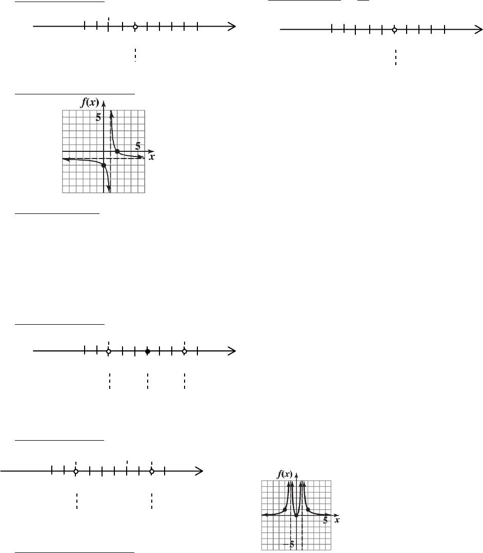
()
x
fx
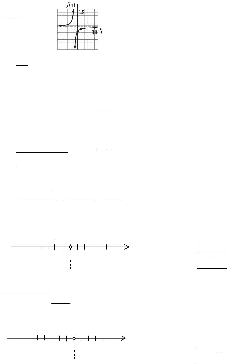
26. f(x) = 2
3
x
x
Step 1. Analyze f(x):
(A) Domain: All real numbers except x = 3.
(B) Intercepts: y-intercept: f(0) = 2
3
x
x
(C) Asymptotes:
x
x
Step 2. Analyze f ꞌ(x):
f ꞌ(x) = 2
(3 ) (2 )
(3 )
x
x
x
= 2
32
(3 )
x
x
x
= 2
5
(3 )
x
= 5(3 – x)–2
x
Step 3. Analyze f“(x):
f“(x) = 10(3 – x)–3 = 3
10
(3 )
x
x
11-36 CHAPTER 11: GRAPHING AND OPTIMIZATION
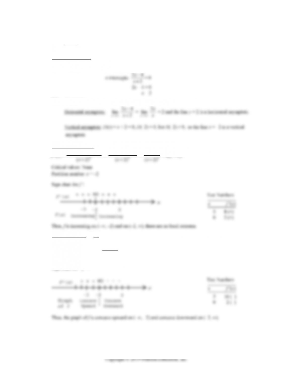
Step 4. Sketch the graph of f:
()
x
fx
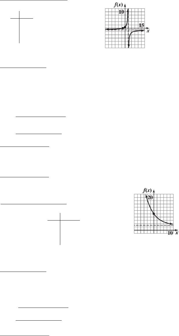
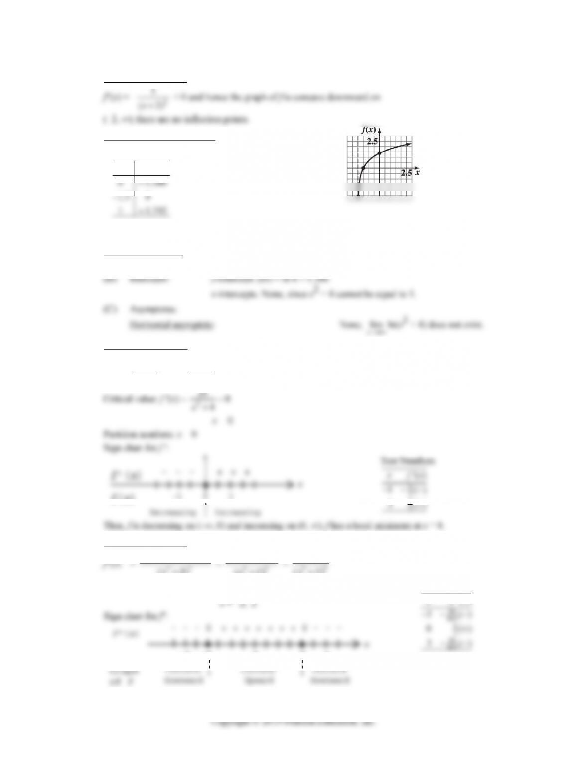
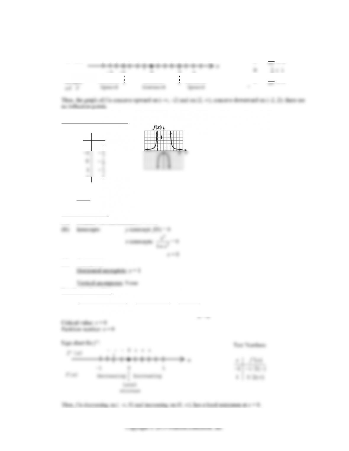
28. f(x) = 3 + 7e–0.2x
Step 1. Analyze f(x):
(A) Domain: All real numbers, (–∞, ∞).
Step 2. Analyze f ꞌ(x):
Step 3. Analyze f“(x):
()
1 11.55
010
x
fx
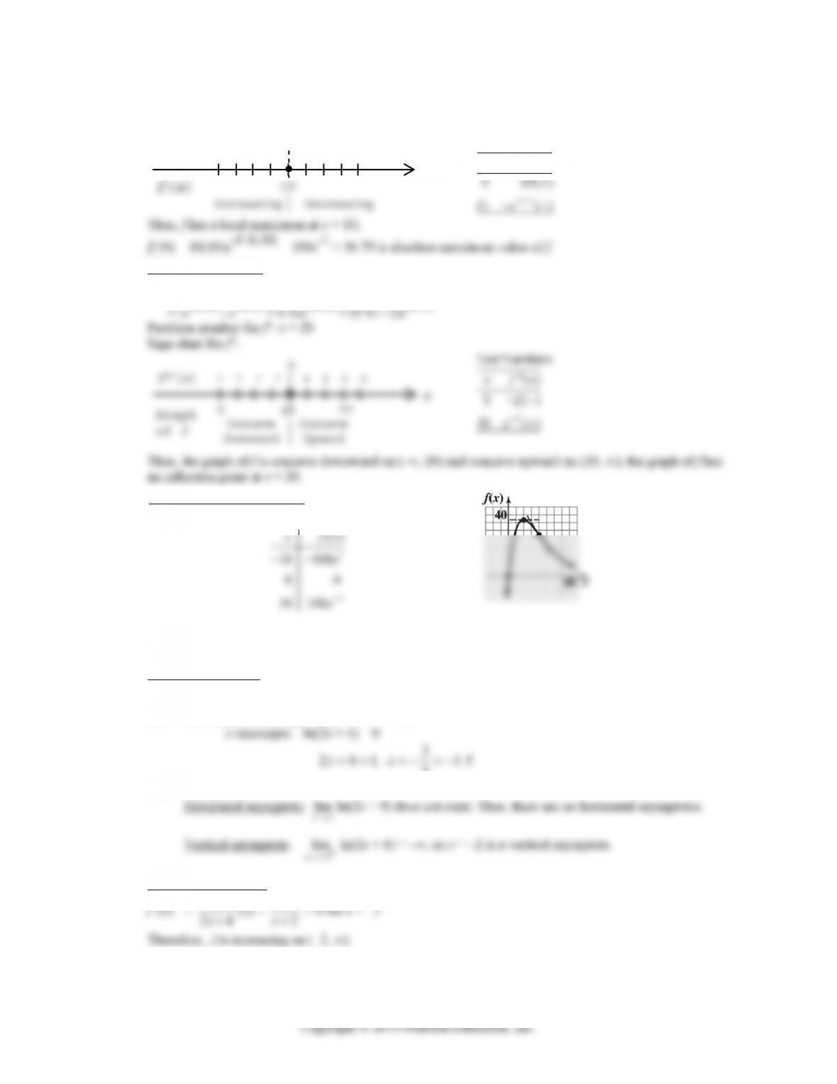
30. f(x) = 10xe–0.1x
Step 1. Analyze f(x):
(A) Domain: All real numbers, (–∞, ∞)
Step 2. Analyze f ꞌ(x):
EXERCISE 11-4 11-37
x = 10 is also a partition number for f ꞌ.
Sign chart for f ꞌ:
+ + + + – – – –
f‘(x)
x
0
Test Numbers
‘( )
x
fx
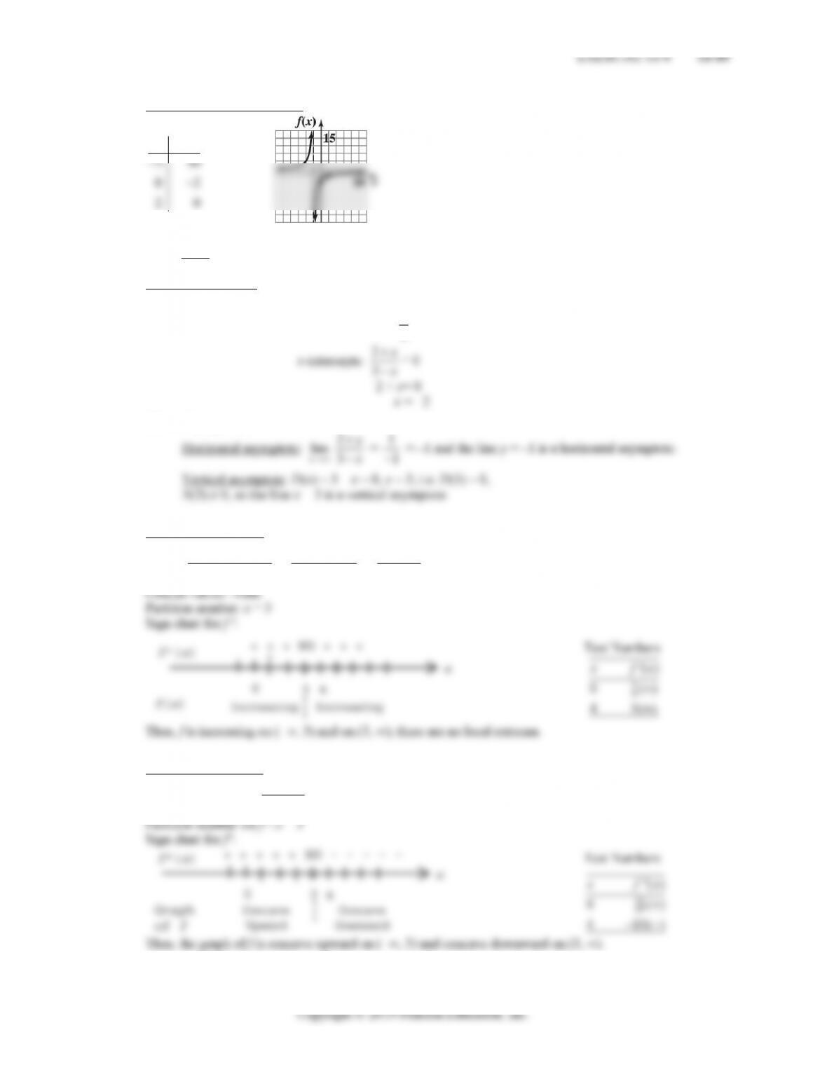
Step 3. Analyze f“(x):
f“(x) = 10(–0.1)e–0.1x – e–0.1x – x(–0.1)e–0.1x
Step 4. Sketch the graph of f:
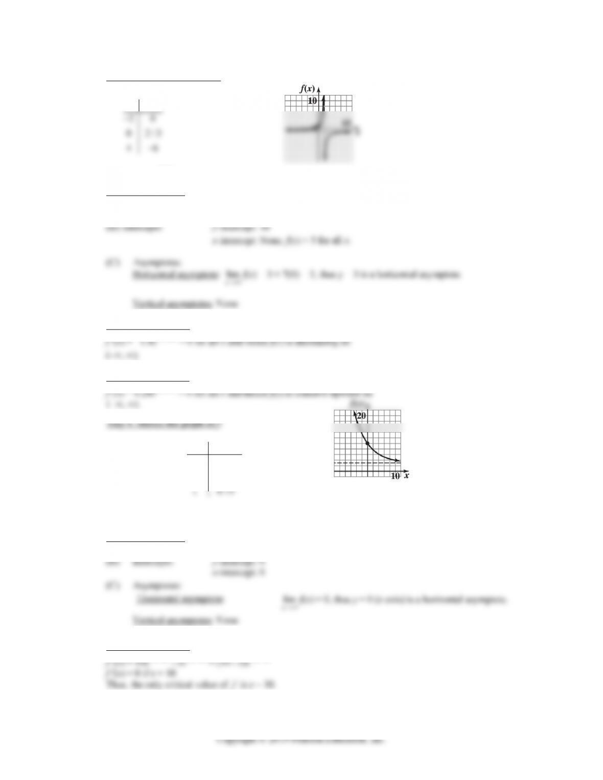
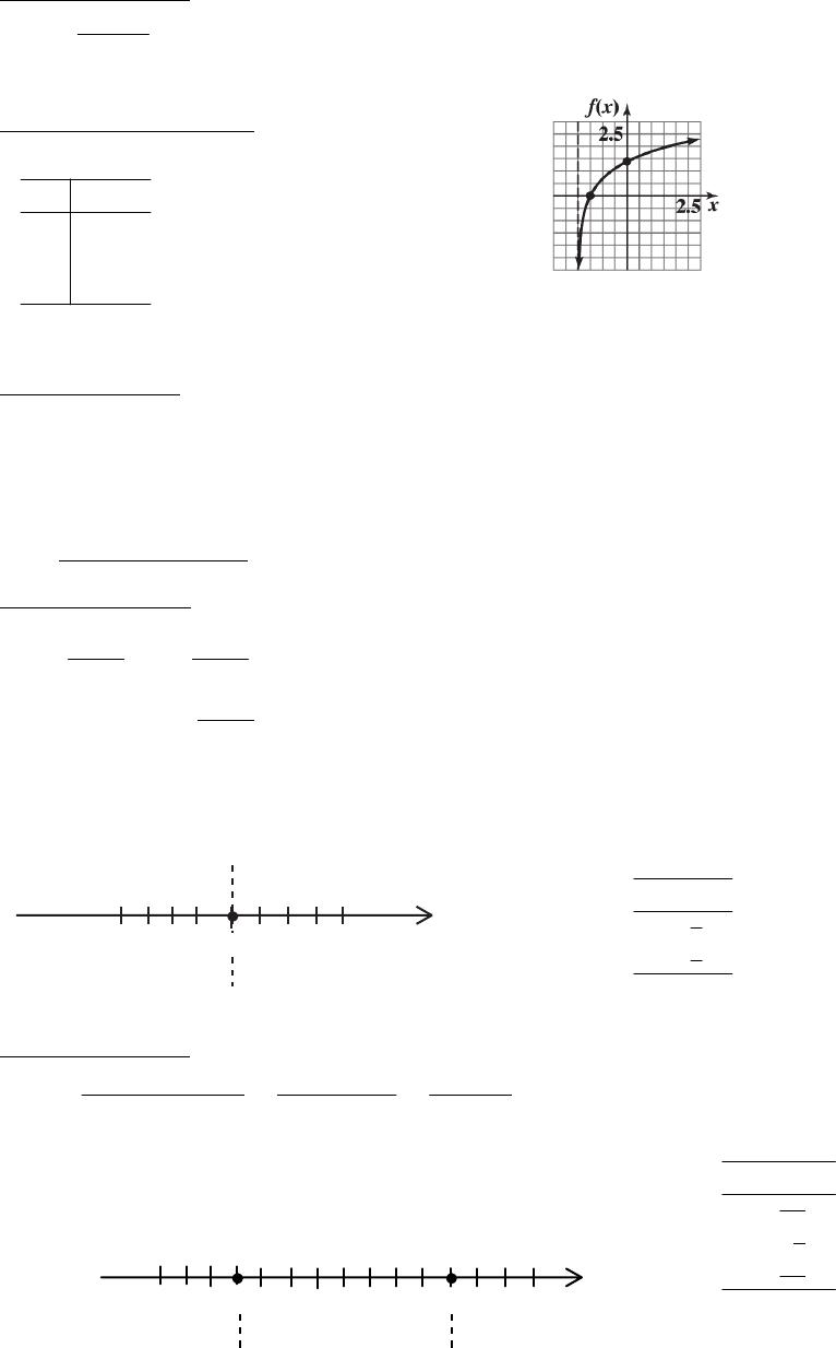
32. f(x) = ln(2x + 4)
Step 1. Analyze f(x):
(A) Domain: 2x + 4 > 0 or x > –2, (–2, ∞)
(B) Intercepts: y-intercept: f(0) = ln 4 ≈ 1.386
2
(C) Asymptotes:
Step 2. Analyze f ꞌ(x):
11-38 CHAPTER 11: GRAPHING AND OPTIMIZATION
Step 3. Analyze f“(x):
Step 4. Sketch the graph of f:
()
x
fx
34. f(x) = ln(x2 + 4)
Step 1. Analyze f(x):
(A) Domain: All real numbers, (–∞, ∞).
Step 2. Analyze f ꞌ(x):
f ꞌ(x) = 2
1
4x(2x) = 2
2
4
x
x
x
f
x
f
(
x
)
-1 1
0
2
x
Step 3. Analyze f“(x):
2
2( 4) 2(2)
(4)
x
xx
x
=
22
284
(4)
x
x
x
=
2
2(4 )
(4)
x
x
Partition numbers for f“: 4 – x2 = (2 – x)(2 + x) = 0
3
-3 0 2
-2
Test Numbers
“( )
x
fx
EXERCISE 11-4 11-39
Step 4. Sketch the graph of f:
()
01.386
x
fx
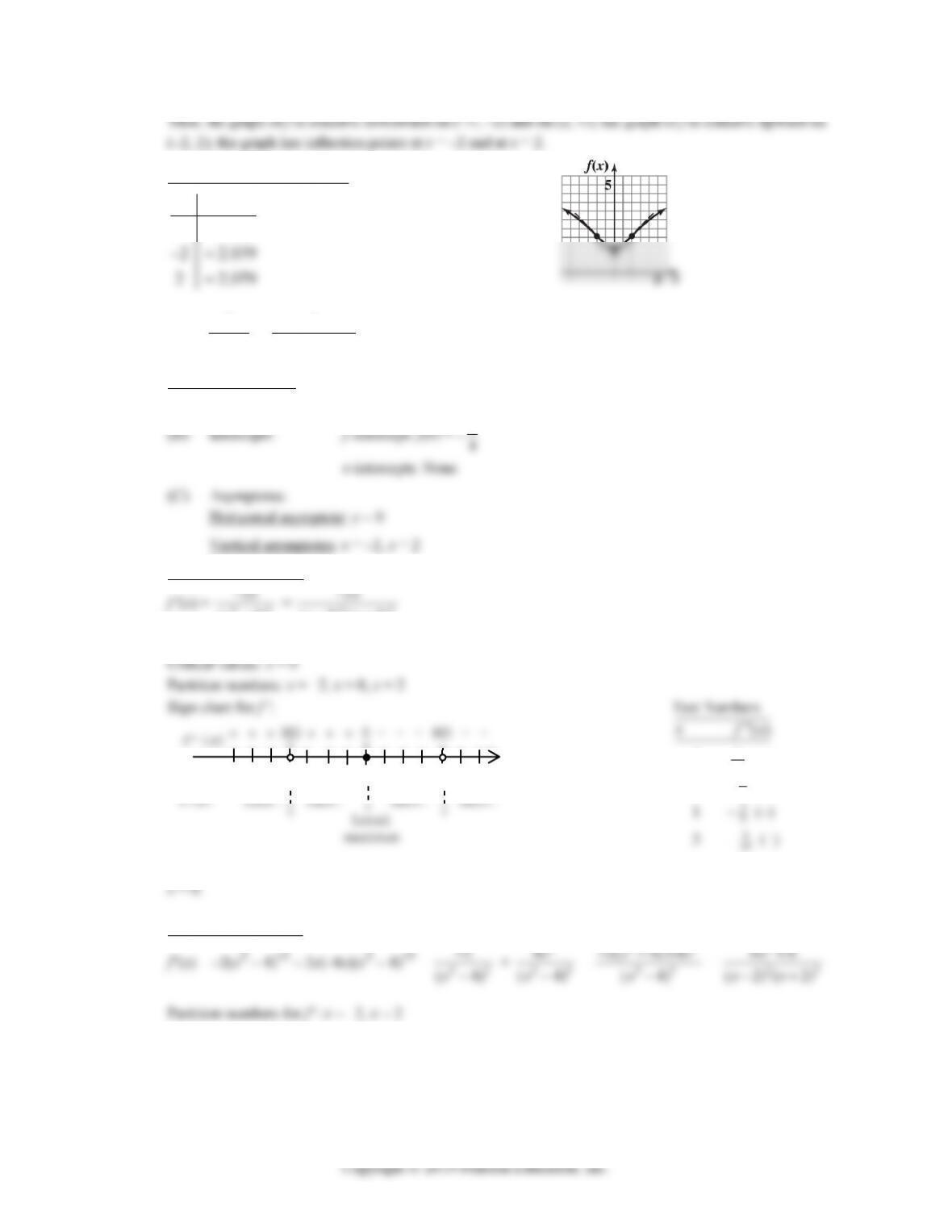
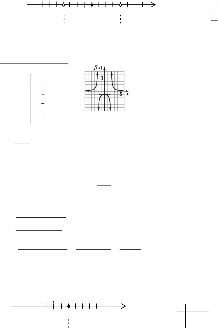
36. f(x) = 2
1
4x = 1
(2)(2)xx
Step 1. Analyze f(x):
(A) Domain: All real numbers except x = –2, x = 2.
Step 2. Analyze f ꞌ(x):
(4)
x
= 22
(2)(2)
xx
f ꞌ(x) = 0 if x = 0
x
-2 1
0
-3 -1 23
–3 6
25 (+)
–1 2
9 (+)
Thus, f is increasing on (–∞, –2) and (–2, 0); decreasing on (0, 2) and (2, ∞); f has a local maximum at
Step 3. Analyze f“(x):
2
22
2
11-40 CHAPTER 11: GRAPHING AND OPTIMIZATION
Sign chart for f“:
3
+ + + ND – – – – – – ND + + +
f“(x)
Concave
Concave
-3 0 2
Concave
-2
Test Numbers
–362
8 (–)
3 62
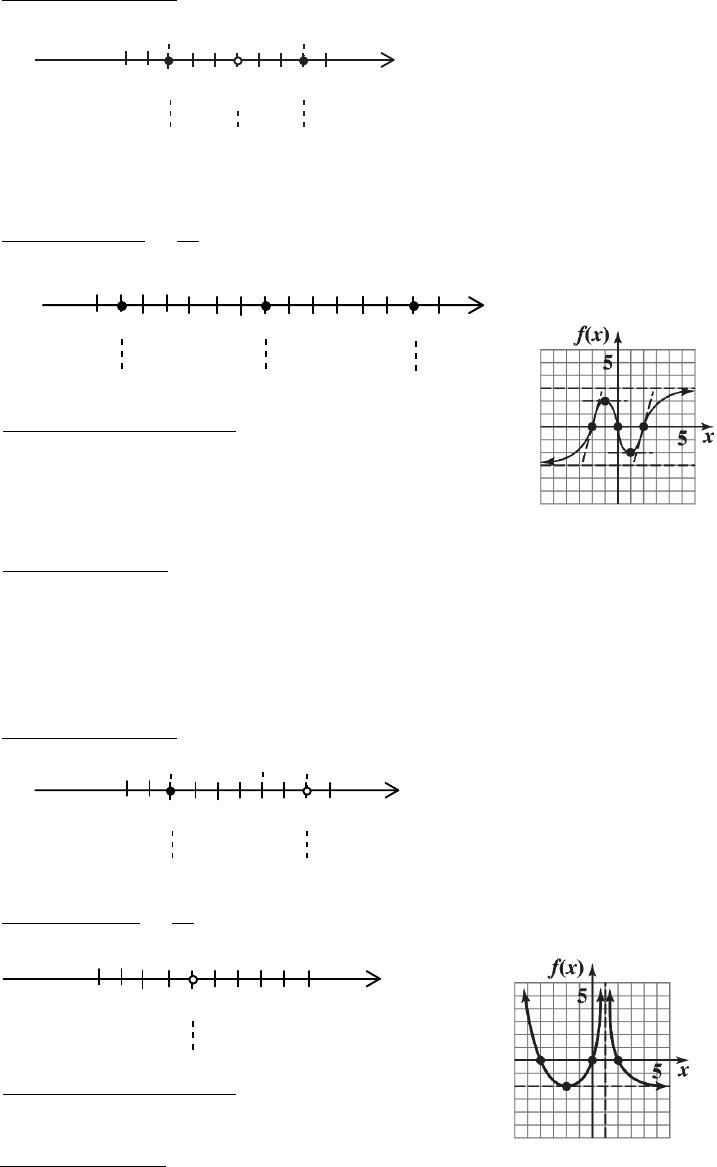
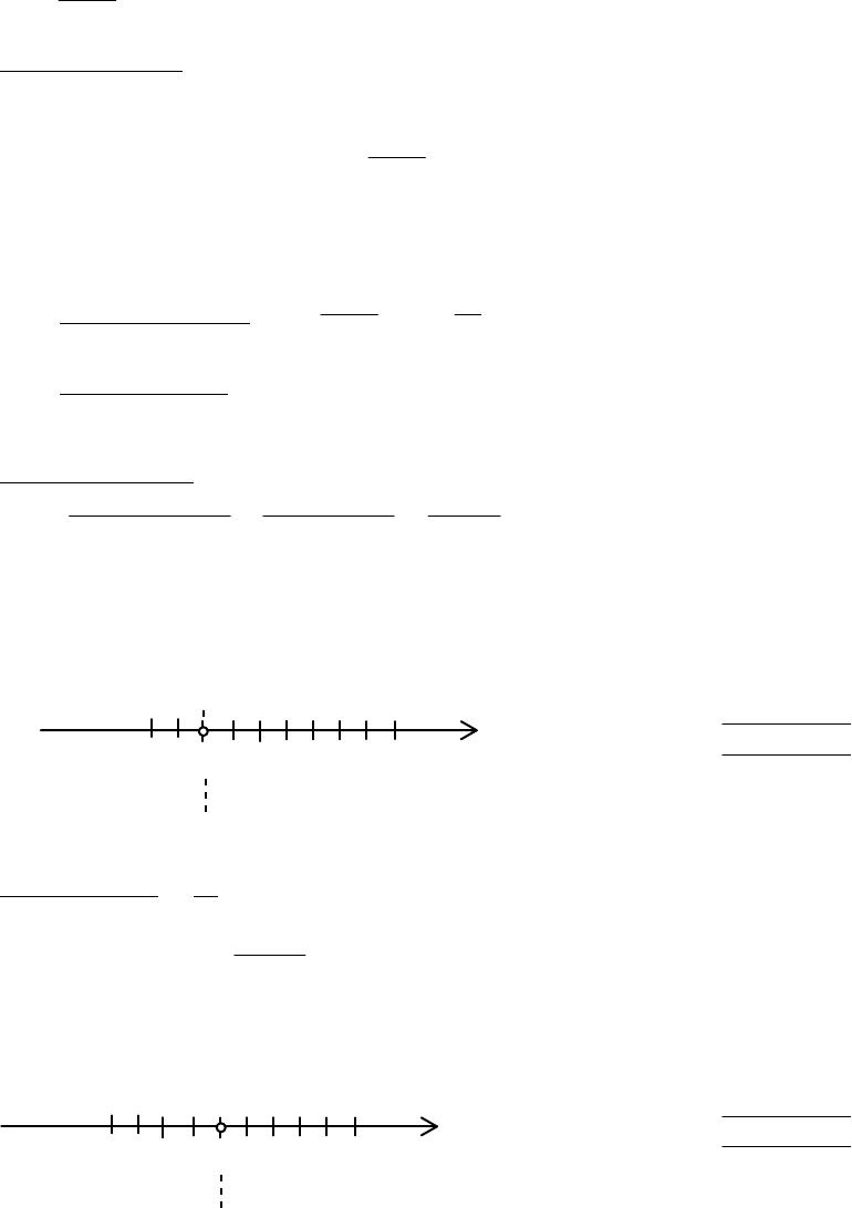
Step 4. Sketch the graph of f:
1
5
1
5
()
3
3
x
fx
38. f(x) =
2
2
1
x
x
Step 1. Analyze f(x):
(A) Domain: All real numbers, (–∞, ∞)
x
x
(C) Asymptotes:
Step 2. Analyze f ꞌ(x):
f ꞌ(x) =
22
22
(2 )(1 ) 2 ( )
(1 )
x
xxx
x
=
33
22
22 2
(1 )
x
xx
x
= 22
2
(1 )
x
x= 0
x