Chapter 11 – Aggregate Planning and Master Scheduling
CHAPTER 11
AGGREGATE PLANNING AND MASTER SCHEDULING
Teaching Notes
In the earlier chapters, we have looked at certain problems that involve long range planning such as
facility location, layout and major equipment purchase decisions. Aggregate planning involves medium
range planning. The planning horizon for medium range plans varies from a couple of months to 18
months. A major component of aggregate planning is to plan aggregate production and inventory levels to
We use the term aggregate plan in lieu of medium range production plan for two reasons:
2. It aggregates daily or weekly (short-range) demand and the resulting production plan (aggregation
of time periods).
Even though the aggregate plan is a function of many different factors, the key factor is the forecasted
demand over the length of the medium-range planning horizon. After developing an aggregate plan
consistent with the forecasted demand and capacity, it is disaggregated into shorter time periods. The
process of disaggregation is the beginning of short range planning using master scheduling and operations
Answers to Discussion and Review Questions
1. Three levels of planning that involve operations managers are:
a. Business plan: It establishes production and capacity strategies.
2. The three phases are forecasting demand, aggregate planning, and disaggregating the overall plan.
Chapter 11 – Aggregate Planning and Master Scheduling
11-2
3. Aggregate planning involves developing a general plan for employment, output, and inventory
4. The need for aggregate planning is to begin to translate long-term decisions into short-term
operating plans. Aggregate planning constitutes the intermediate step in this process.
6. The difficulty relates to finding a common unit on which to base aggregate plans when there are a
variety of products or services to contend with.
7. a. Maintaining a constant workforce has the advantage of making estimation of labor costs
relatively easy, is good for morale, and minimizes hiring and layoff costs. However,
9. a. Spreadsheets are intuitively appealing and easy to understand, but solutions are not
necessarily optimal.
b. Linear Programming (LP): LP approach is a method of obtaining optimal solutions to problems
involving allocation of limited resources. The objective of linear programming is either
10. The master schedule has three inputs: the beginning inventory, forecasts for each period of the
11. Aggregate planning helps managers establish plans for inputs and outputs and employment level
and budgets for the intermediate term. The plans involve collaboration among finance,
Chapter 11 – Aggregate Planning and Master Scheduling
11-3
Taking Stock
1. When we freeze a portion of the master schedule, we make the schedule more stable and reduce
2. Purchasing agents, production planning and control manager, planners, schedulers, and marketing
personnel need to interface with the master schedule. Purchasing agents, planners and schedulers
need direct information from the MPS to order the parts, manage the inventories of the parts and
3. The new communication tools made it easier to communicate changes in the master schedule.
Therefore, when a change is necessary in the master schedule (addition or a deletion of an order,
change in the due date or the quantity of an order), it can be communicated to the master
Critical Thinking Exercise
1. Compared to manufacturing environments, service environments often experience more
pronounced variations in demand over shorter time intervals. Moreover, employing inventory as a
2. Student answers will vary.
Memo Writing Exercise
1. Aggregate Planning is the planning of the overall, general use of resources based on expected
Chapter 11 – Aggregate Planning and Master Scheduling
11-4
Aggregate Planning determines the level of output for a given service or product by managing the
2. Chase strategy matches production with varying demand rates. This strategy involves either
varying the workforce levels or varying the capacity by using either overtime or subcontracting.
The primary advantage of using Chase strategy is that inventory carrying cost is minimized. The
main disadvantage is the additional cost of changing the workforce level (hiring, layoffs and
employee morale) or the cost of overtime/subcontracting.
Chapter 11 – Aggregate Planning and Master Scheduling
Solutions
1.
From example 1.
Period
1
2
3
4
5
6
Total
Forecast
200
200
300
400
500
200
1,800
Output
Regular
300
300
300
0
450
450
1,800
Overtime
Subcontract
Output-
Forecast
100
100
0
(400)
(50)
250
Inventory
Beginning
0
100
200
200
0
0
Ending
100
200
200
0
0
0
Average
50
150
200
100
0
0
500
Backlog
0
0
0
200
250
0
450
Costs:
Output
Regular
$600
600
600
0
900
900
3,600
Overtime
Subcontract
Inventory
50
150
200
100
0
0
500
Backorder @ 5
0
0
0
1,000
1,250
0
2,250
Total
$650
750
800
1,100
2,150
900
6,350
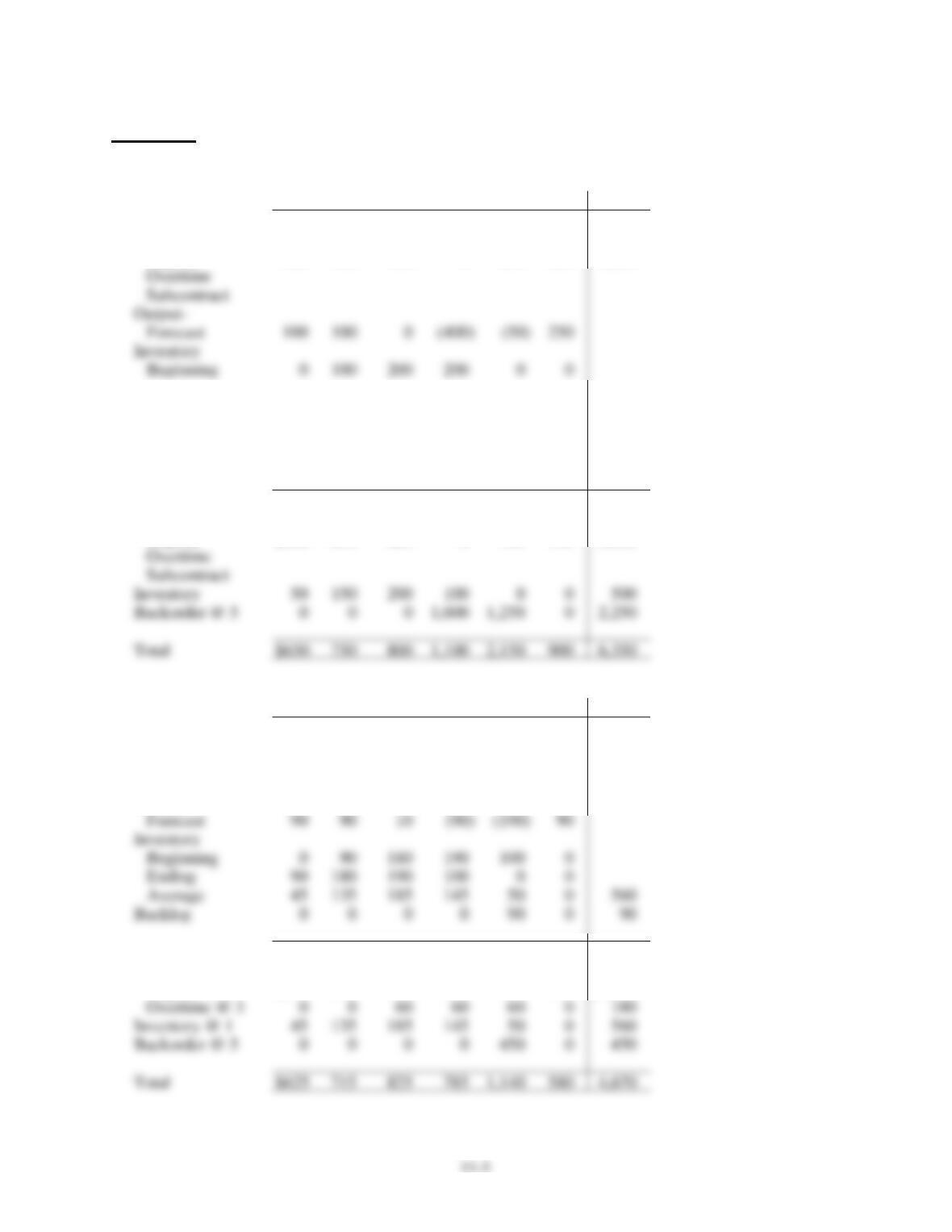
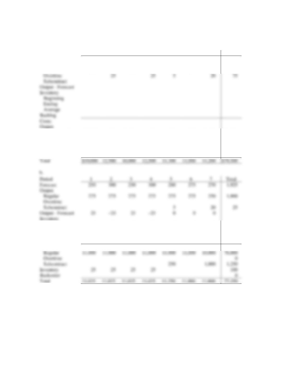
2. a. (Other plans are possible)
Period
1
2
3
4
5
6
Total
Forecast
200
200
300
400
500
200
1,800
Output
Regular
290
290
290
290
290
290
1,740
Overtime
20
20
20
60
Output-
Forecast
90
90
10
(90)
(190)
90
Inventory
Beginning
0
90
180
190
100
0
Ending
90
180
190
100
0
0
Backlog
0
0
0
0
90
0
90
Costs:
Regular @ 2
$580
580
580
580
580
580
$3,480
Overtime @ 3
0
0
60
60
60
0
180
Inventory @ 1
45
135
185
145
50
0
560
Backorder @ 5
0
0
0
0
450
0
450
Chapter 11 – Aggregate Planning and Master Scheduling
11-6
2. b. (Other plans are possible)
Period
1
2
3
4
5
6
Total
Forecast
200
200
300
400
500
200
1,800
Output
Regular
290
290
290
290
290
290
1,740
Subcontract
10
50
60
Costs:
Regular @ 2
$580
580
580
580
580
580
$3,480
Subcontract @ 6
0
0
0
60
300
0
360
Inventory @ 1
45
135
175
120
35
0
510
Backorder @ 5
0
0
0
0
450
0
450
Total
$625
715
755
760
1,365
580
$4,800
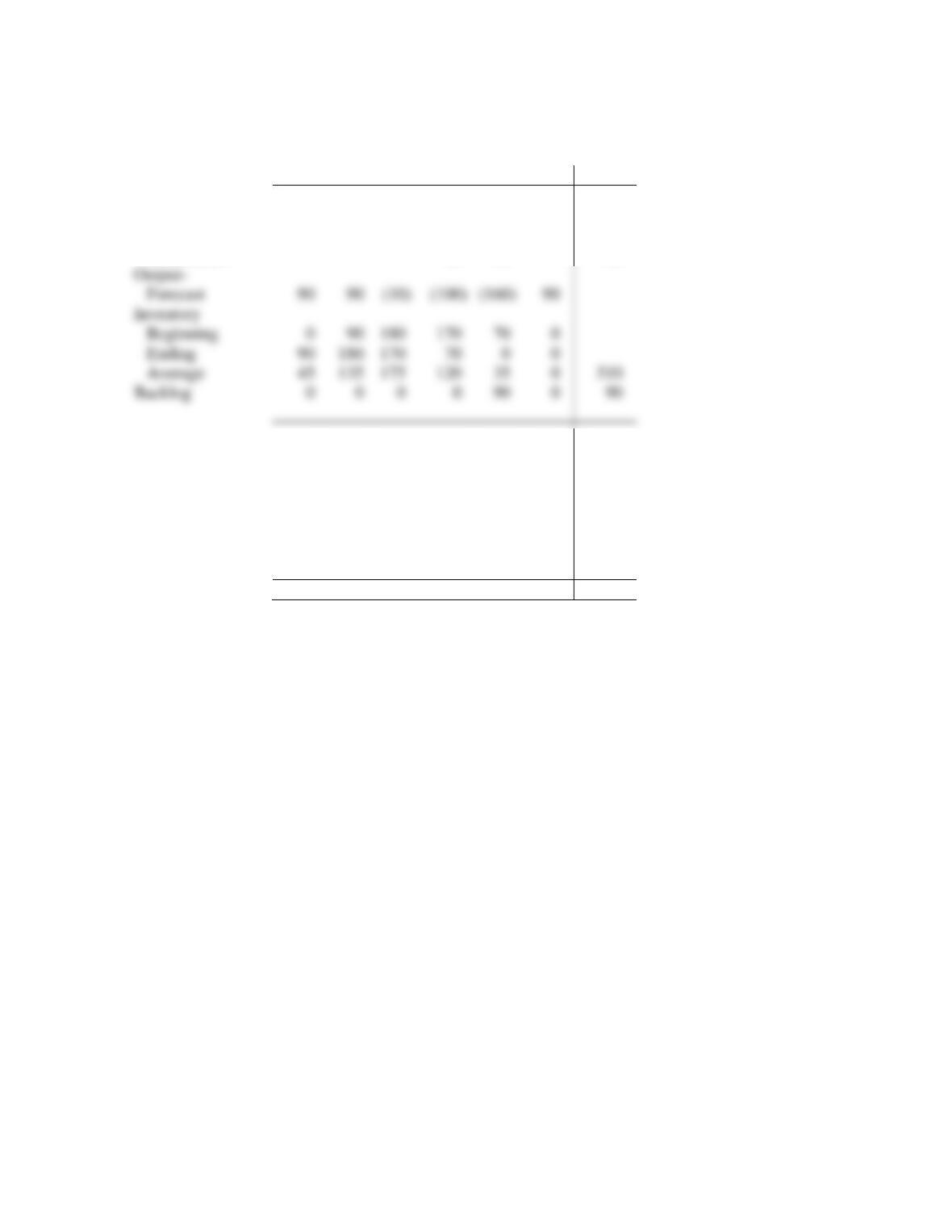
Output-
Forecast
90
90
(100)
(160)
90
Inventory
Beginning
90
180
170
70
0
Ending
90
180
170
70
0
0
Backlog
0
90
0
Chapter 11 – Aggregate Planning and Master Scheduling
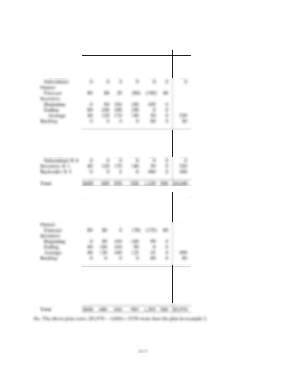
3.
Period
1
2
3
4
5
6
Total
Forecast
200
200
300
400
500
200
1,800
Output
Regular
280
280
280
280
280
280
1,680
Overtime
0
0
40
40
40
0
120
Subcontract
0
0
0
0
0
0
Output-
Forecast
80
80
20
(180)
80
Inventory
Beginning
0
80
160
180
100
0
Ending
80
160
180
100
0
0
Average
40
120
170
140
50
0
520
Backlog
0
0
0
0
80
0
Costs:
Output
Regular @ 2
$560
560
560
560
560
560
$3,360
Overtime @ 3
0
0
120
120
120
0
360
Subcontract @ 6
0
0
0
0
0
0
Inventory @ 1
40
120
170
140
50
0
520
Backorder @ 5
0
0
0
0
400
0
400
Total
$600
680
850
820
1,120
560
$4,640
4.
Period
1
2
3
4
5
6
Total
Forecast
200
200
300
400
500
200
1,800
Output
Regular
280
280
280
280
280
280
1,680
Subcontract
0
0
20
50
50
0
120
Output-
Forecast
80
80
0
(170)
80
Inventory
Beginning
0
80
160
160
90
0
Ending
80
160
160
90
0
0
Average
40
120
160
125
45
0
490
Backlog
0
0
0
0
80
0
Costs:
Regular @ 2
$560
560
560
560
560
560
$3,360
Subcontract @ 6
0
0
120
300
300
0
720
Inventory @ 1
40
120
160
125
45
0
490
Backorder @ 5
0
0
0
0
400
0
400
Total
$600
680
840
985
1,305
560
$4,970
Chapter 11 – Aggregate Planning and Master Scheduling
11-8
5. a.
Period
1
2
3
4
5
6
7
8
Total
Forecast
120
135
140
120
125
125
140
135
1,040
Output
Regular
120
130
130
120
125
125
130
130
1,010
Regular @ 60
$7,200
7,800
7,800
7,200
7,500
7,500
7,800
7,800
$60,600
Overtime @ 90
450
900
900
450
2,700
Subcontract
Inventory @ 5
Backorder
Total
7,200
7,200
7,500
7,500
8,700
$63,300
Period
1
2
3
4
5
6
7
8
Total
Forecast
Output
Regular
130
130
130
130
130
130
130
130
1,040
Overtime
Subcontract
Output – Forecast
10
(10)
5
5
(10)
Inventory
Beginning
0
10
5
0
5
10
15
5
Ending
10
5
0
5
10
15
5
0
Average
5
7.5
2.5
2.5
7.5
12.5
10
2.5
Backlog
5
Costs:
Output
Regular @ 60
7,800
7,800
7,800
7,800
7,800
7,800
7,800
$62,400
Overtime
Subcontract @ 50
Inventory @ $2
Backorder @ $90
450
Total
$62,950
Overtime
10
Subcontract
Output – Forecast
0
(10)
0
0
0
(10)
Inventory
Beginning
Ending
Average
Backlog
Costs:
Output
Chapter 11 – Aggregate Planning and Master Scheduling
11-9
6. a.
Period
1
2
3
4
5
6
7
Total
Forecast
250
300
250
300
280
275
270
Output
Regular
250
275
250
275
275
275
250
1,850
Regular @ 40
$10,000
11,000
10,000
11,000
11,000
11,000
10,000
$74,000
Overtime @ 60
1,500
1,500
300
1,200
4,500
Subcontract
Inventory
Backorder
Total
$10,000
$78,500
Period
1
2
3
4
5
6
7
Total
Forecast
Output
Regular
275
275
275
275
275
275
250
1,900
Overtime
Subcontract
5
20
25
Output – Forecast
25
25
0
0
0
Inventory
Beginning
0
25
0
25
0
0
0
Ending
25
0
25
0
0
0
0
Average
12.5
12.5
12.5
12.5
0
0
0
50
Backlog
0
0
0
0
0
0
0
0
Costs:
Regular
11,000
11,000
11,000
11,000
11,000
11,000
10,000
Overtime
0
Subcontract
250
1,000
1,250
Inventory
25
25
25
25
Backorder
0
Total
11,025
11,025
11,025
11,025
11,250
11,000
11,000
Overtime
25
25
5
20
75
Subcontract
Output – Forecast
Inventory
Beginning
Ending
Average
Backlog
Costs:
Output
Chapter 11 – Aggregate Planning and Master Scheduling
11-10
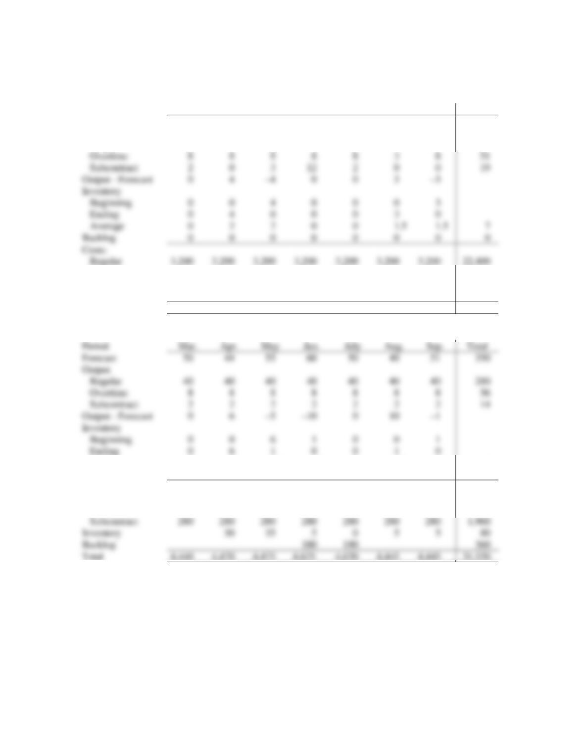
7. a. No backlogs are allowed
Period
Mar.
Apr.
May
Jun.
July
Aug.
Sep.
Total
Forecast
50
44
55
60
50
40
51
350
Output
Regular
40
40
40
40
40
40
40
280
Overtime
960
960
960
960
960
360
960
6,120
Subcontract
280
0
420
1,680
280
0
0
2,660
Inventory
0
20
20
0
0
15
15
70
Total
4,440
4,180
4,600
5,840
4,440
3,575
4,175
31,250
b. Level strategy
Period
Mar.
Apr.
May
Jun.
July
Aug.
Sep.
Total
Forecast
50
44
55
60
50
40
51
350
Output
Regular
40
40
40
40
40
40
40
280
Overtime
8
8
8
8
8
8
8
56
Subcontract
2
2
2
2
2
2
2
14
Output – Forecast
0
6
0
10
Inventory
Beginning
0
0
6
1
0
0
1
Ending
0
6
1
0
0
1
0
Average
0
3
3.5
.5
0
.5
.5
8
Backlog
0
0
0
9
9
0
0
18
Costs:
Regular
3,200
3,200
3,200
3,200
3,200
3,200
3,200
22,400
Overtime
960
960
960
960
960
960
960
6,720
Subcontract
280
280
280
280
280
280
280
1,960
Inventory
30
35
5
0
5
5
80
Backlog
180
180
360
Total
4,440
4,470
4,475
4,625
4,620
4,445
4,445
31,520
Overtime
8
8
8
8
8
3
8
51
Subcontract
2
0
3
12
2
0
0
19
Output – Forecast
0
4
0
0
3
Inventory
Beginning
0
0
4
0
0
0
3
Ending
0
4
0
0
0
3
0
Average
0
2
2
0
0
1.5
1.5
7
Backlog
0
0
0
0
0
0
0
0
Costs:
Regular
3,200
3,200
3,200
3,200
3,200
3,200
3,200
22,400
Chapter 11 – Aggregate Planning and Master Scheduling
11-11
8. a. Level production supplemented with overtime as needed.
Period
1
2
3
4
5
6
Total
Forecast
4,000
4,800
5,600
7,200
6,400
5,000
33,000
Output
Regular
5,000
5,000
5,000
5,000
5,000
5,000
30,000
Inventory @ 1
500
1,100
900
300
0
0
2,800
Back orders @ 10
0
0
0
0
0
0
0
Total
50,500
51,100
50,900
75,900
72,400
50,000
350,800
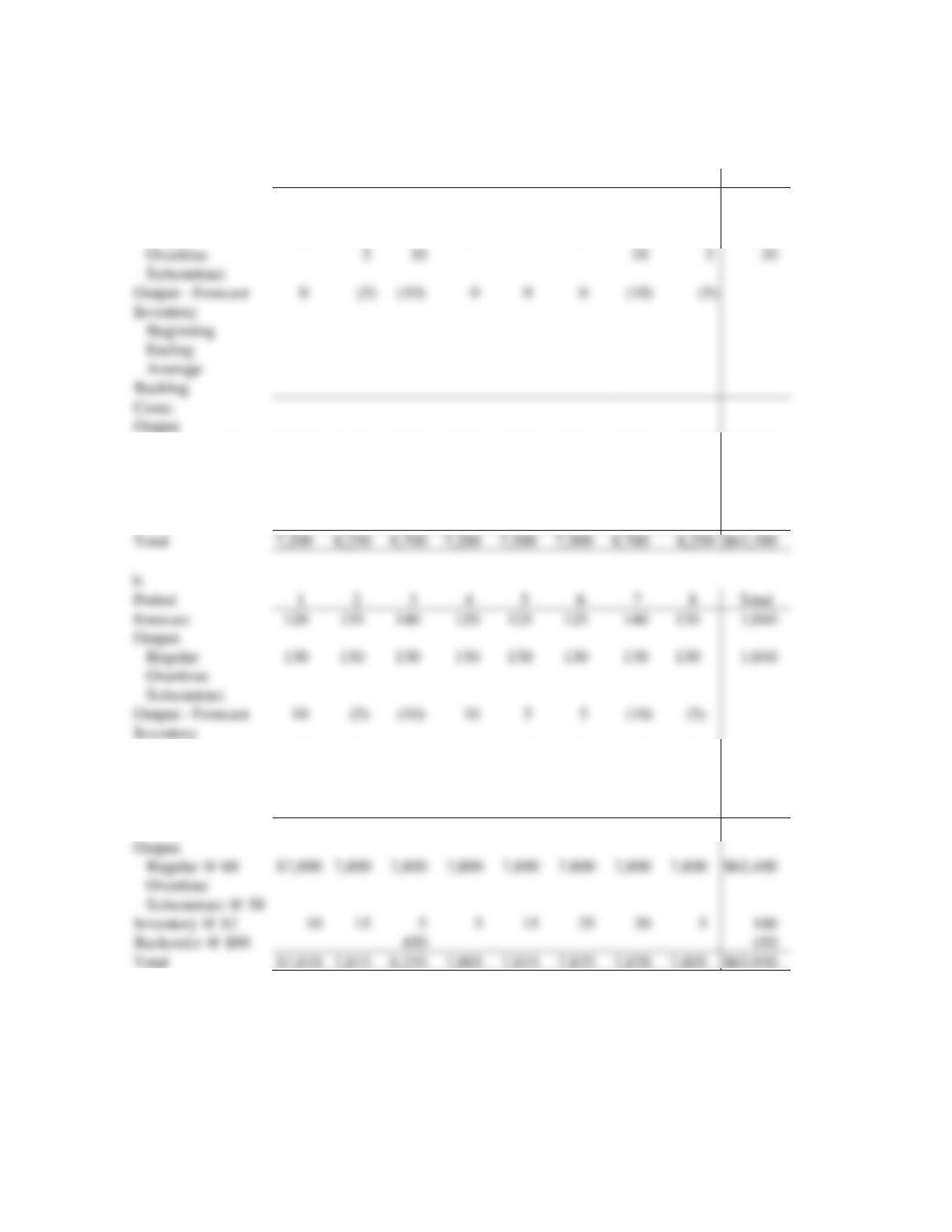
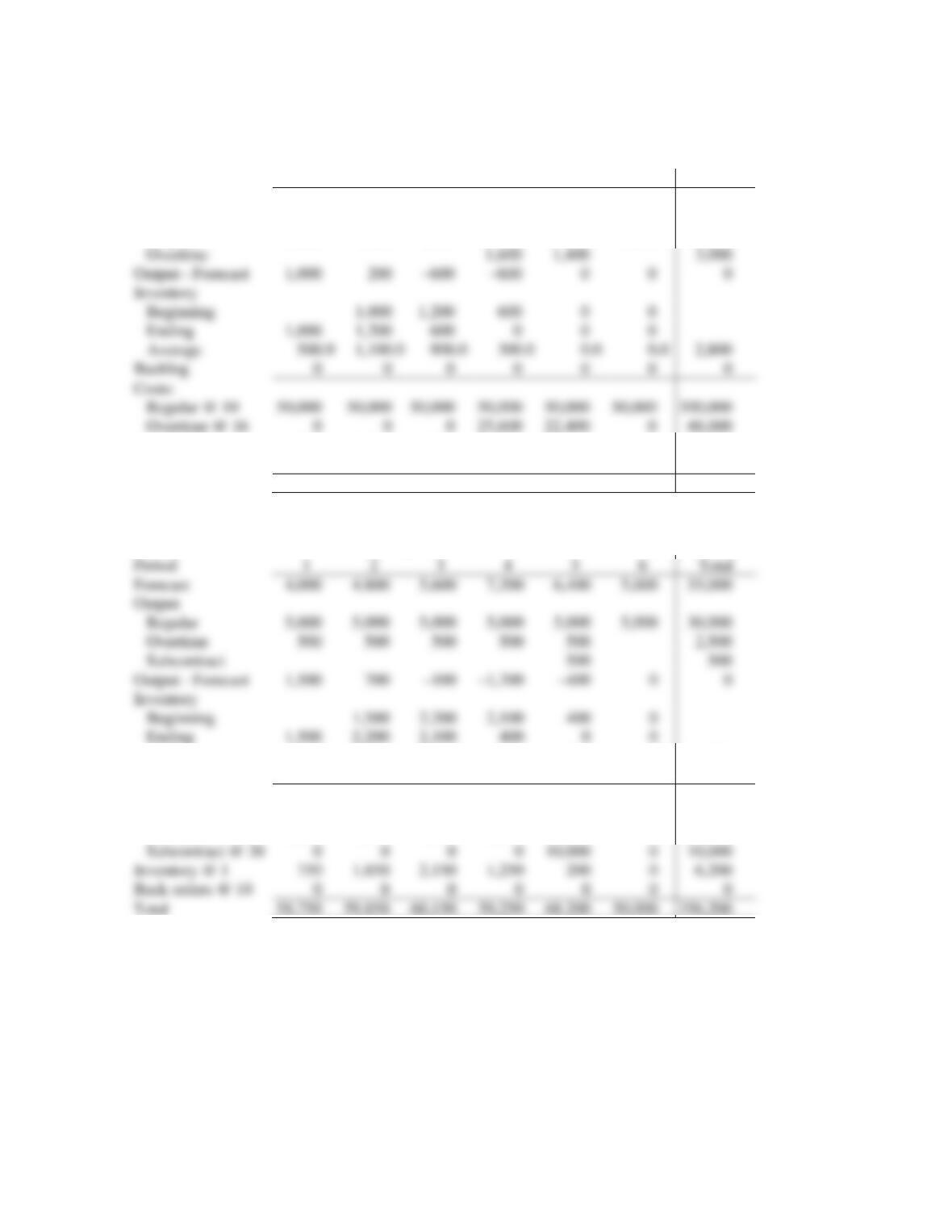
b. Combination of overtime, inventory and subcontracting to handle variations in demand. Max.
overtime = 500, max. subcontracting = 500 units.
Period
1
2
3
4
5
6
Total
Forecast
Output
Regular
5,000
5,000
5,000
5,000
5,000
5,000
30,000
Overtime
500
500
500
500
2,500
Subcontract
500
Output – Forecast
1,500
0
0
Inventory
Beginning
1,500
2,200
2,100
400
0
Ending
1,500
2,200
2,100
400
0
0
Average
750.0
1,850.0
2,150.0
1,250.0
200.0
0.0
6,200
Backlog
0
0
0
0
0
0
0
Costs:
Regular @ 10
50,000
50,000
50,000
50,000
50,000
50,000
300,000
Overtime @ 16
8,000
8,000
8,000
8,000
8,000
0
40,000
Subcontract @ 20
0
0
0
0
10,000
0
10,000
Inventory @ 1
750
1,850
2,150
1,250
200
0
6,200
Back orders @ 10
0
0
0
0
0
0
0
Total
356,200
Overtime
1,600
1,400
3,000
Output – Forecast
1,000
0
0
0
Inventory
Beginning
1,000
1,200
600
0
0
Ending
1,000
1,200
600
0
0
0
Average
500.0
1,100.0
900.0
300.0
0.0
0.0
2,800
Backlog
0
0
0
0
0
0
0
Costs:
Regular @ 10
50,000
50,000
50,000
50,000
50,000
300,000
Overtime @ 16
0
0
0
25,600
22,400
0
48,000
Chapter 11 – Aggregate Planning and Master Scheduling
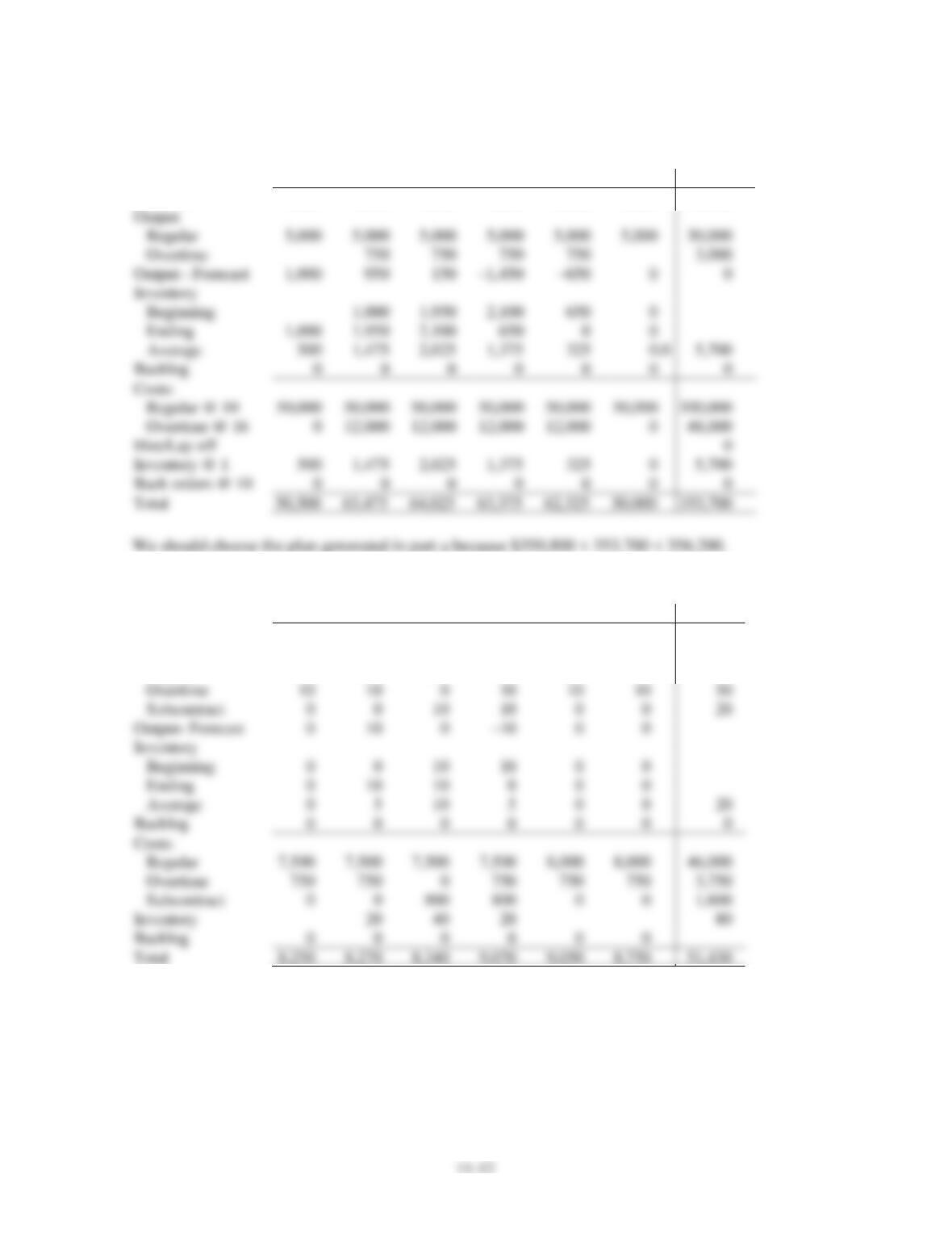
c. Overtime up to 750 units per period maximum to handle variations in demand.
Period
1
2
3
4
5
6
Total
Forecast
4,000
4,800
5,600
7,200
6,400
5,000
33,000
Output
Regular
Overtime
Output – Forecast
Inventory
Beginning
Ending
Average
Backlog
Regular @ 10
300,000
Overtime @ 16
Hire/Lay off
Inventory @ 1
Back orders @ 10
9.
Period
1
2
3
4
5
6
Total
Forecast
160
150
160
180
170
140
960
Output
Regular
150
150
150
150
160
160
920
Overtime
Subcontract
Inventory
Beginning
Ending
Average
Backlog
Costs:
Regular
Overtime
750
750
750
750
750
Subcontract
800
800
Inventory
Backlog