Excel Templates to accompany Operations Management, Eleventh Edition
created by Lee Tangedahl
Copyright © 2012 by The McGraw Hill Companies, Inc. All rights reserved.
Chapter Eleven – Aggregate Planning and Master Scheduling
Templates: Aggregate Planning (B) Solved Problems: Solved Problem 1
Problems 14-19
Lecture Suggestions Problems 20-23
Examples: Example 1
Example 2
Example 3
See the Aggregate Planning tutorial for a demonstration of the Aggregate Planning template.
See the Transportation Model tutorial for a demonstration of the Transportation Model template.
See Instructions template for complete instructions.
Transportation Model (Basic) Solved Problem 2
Master Scheduling (B) Solved Problem 3
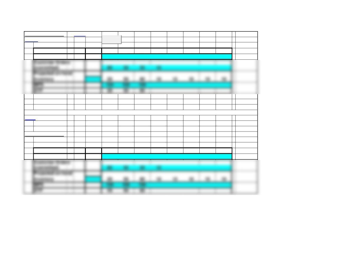
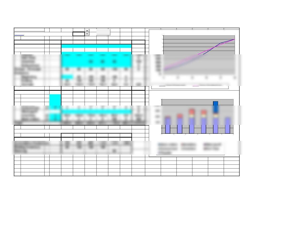
Aggregate Planning
Aggregate Planning
Basic
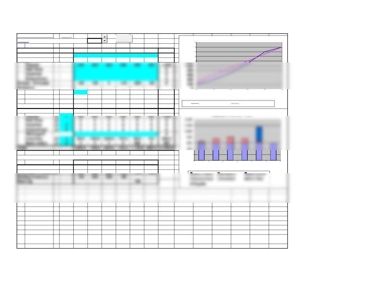
<Back Number of periods: 6
Period 1 2 3 4 5 6 Total
Forecast 200 200 300 400 500 200 1,800
Output
Beginning 100 200 200 100 0
Ending 100 200 200 100 0 0
Average 50.0 150.0 200.0 150.0 50.0 0.0 600
Backlog 0 0 0 0 100 0100
Costs:
Inventory @ 1 50.0 150.0 200.0 150.0 50.0 0.0 600.0
See the Aggregate Planning tutorial for a demonstration of this template.
1 2 3 4 5 6
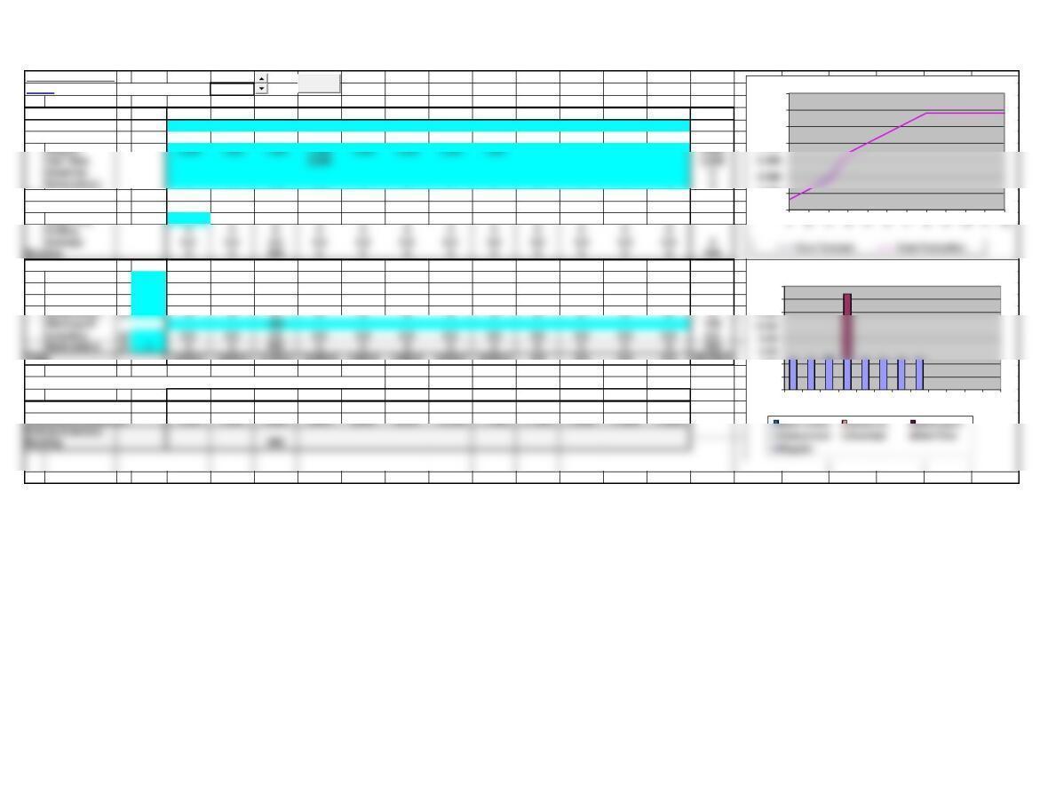
Cumulative Forecast 200 400 700 1,100 1,600 1,800
Cumulative Production
300 600 900 1,200 1,500 1,800
Ending Inventory 100 200 200 100
0
200
1 2 3 4 5 6
Aggregate Planning – Costs
0
1,400
1,600
1,800
2,000
1 2 3 4 5 6
Cum Forecast Cum Production
Clear
Page 2
Output – Forecast 100 100 0-100 -200 100 0
Inventory
Aggregate Planning
Basic Template: You can simply copy the basic template below and paste into another worksheet.
^Top After pasting into another worksheet you should delete unneeded columns.
Aggregate Planning
Period 1 2 3 4 5 6 Total
Forecast 200 200 300 400 500 200 1,800
Output
Regular 300 300 300 300 300 300 1,800
Beginning 100 200 200 100 0
Ending 100 200 200 100 0 0
Average 50.0 150.0 200.0 150.0 50.0 0.0 600
Backlog 0 0 0 0 100 0100
Costs:
Regular @ 2 600 600 600 600 600 600 3,600
Inventory @ 1 50.0 150.0 200.0 150.0 50.0 0.0 600.0
Total 650.0 750.0 800.0 750.0 1,150.0 600.0 4,700.0
Page 3
Output – Forecast 100 100 0-100 -200 100 0
Inventory
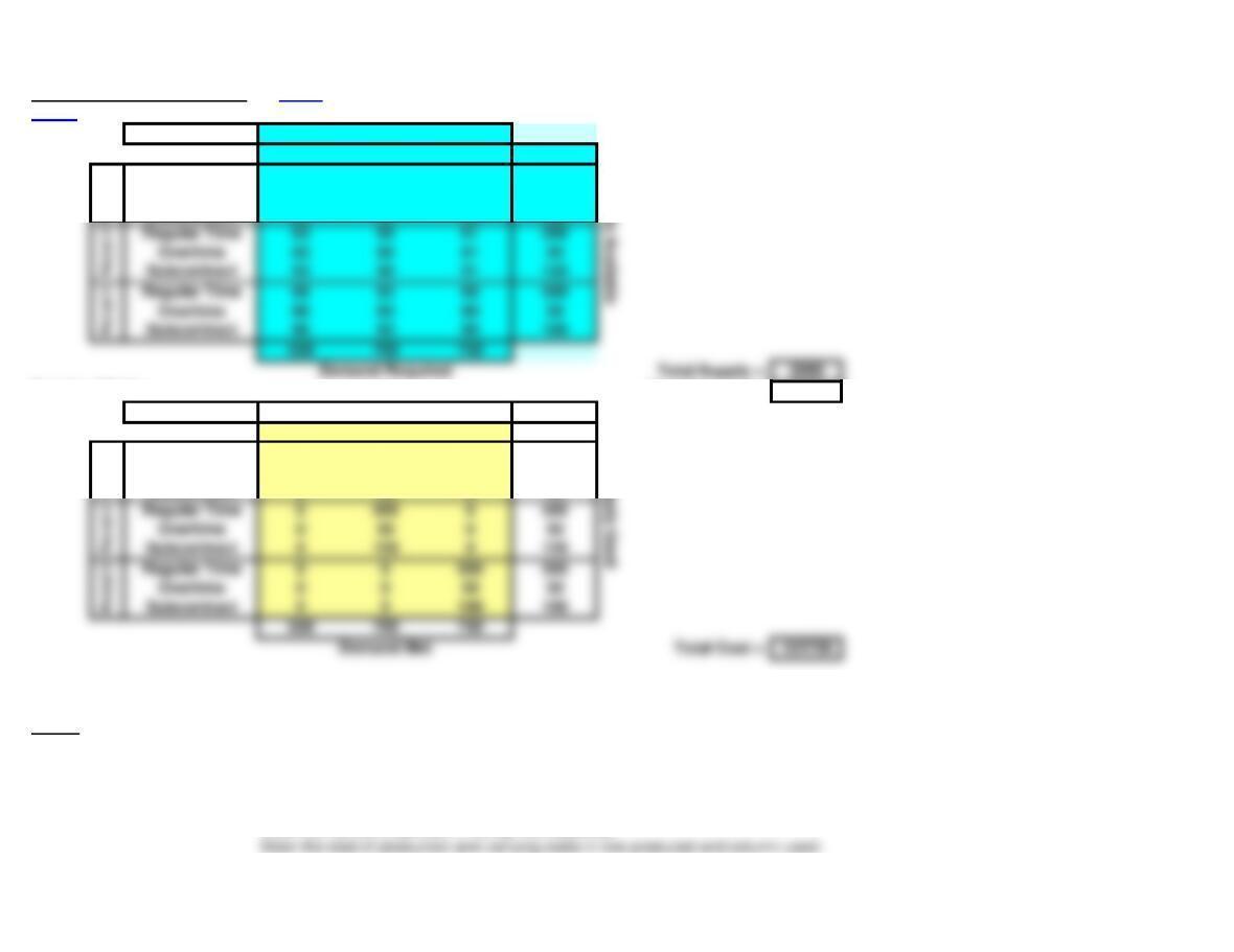
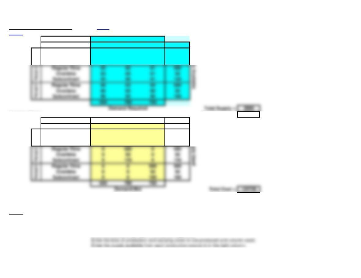
Transportation Model (Basic) Notes Use Solver on Data Ribbon to solve – see notes below.
<Back Do not change or delete unshaded cells.
Input Matrix:
Demand for: Period 1 Period 2 Period 3
Beginning Inventor
0 1 2 100
Regular Time 60 61 62 500
Overtime 80 81 82 50
Subcontract 90 91 92 120
Solution Matrix: Total Demand = 2000
Demand for: Period 1 Period 2 Period 3 0
Beginning Inventor
100 0 0 100
Regular Time 400 0100 500
Overtime 50 0 0 50
Subcontract 0 30 030
Regular Time 0 500 0500
Regular Time 0 0 500 500
Period 2
Period 3
Notes: See the Transportation tutorial for a demonstration of a similar template.
Unneeded rows and columns have been hidden in the above template.
1. Enter the problem into the Input Matrix (top shaded area):
Enter the names of periods in the top row (optional).
Supply Used
Period 1
Supply Available
Period 1
Regular Time 63 60 61 500
Overtime 83 80 81 50
Subcontract 93 90 91 120
Regular Time 66 63 60 500
Overtime 86 83 80 50
Subcontract 96 93 90 100
Period 2
Period 3
2. You can manually create solutions in the Solution Matrix (bottom shaded area):
Enter amounts in the row produced and column used in the middle of the Solution Matrix (shaded yellow).
3. Using Solver to find the optimal solution:
Select the Data ribbon, the Solver Add-in must be available in the Analysis group (see note below to add-in Solver).
Press Solver in the Analysis group of the Data ribbon.
More… 4. Notes on the Solver solution:
Small numbers in scientific notation (e.g. 2.4091E-11) reflect the precision of Solver and can be treated as zero.
If total demand exceeds total supply then problem is not feasible and you will get an error message.
5. How to Add-In Solver if it does not appear in the Analysis group of the Data ribbon:
Select File (left-most item in main menu at top of screen).
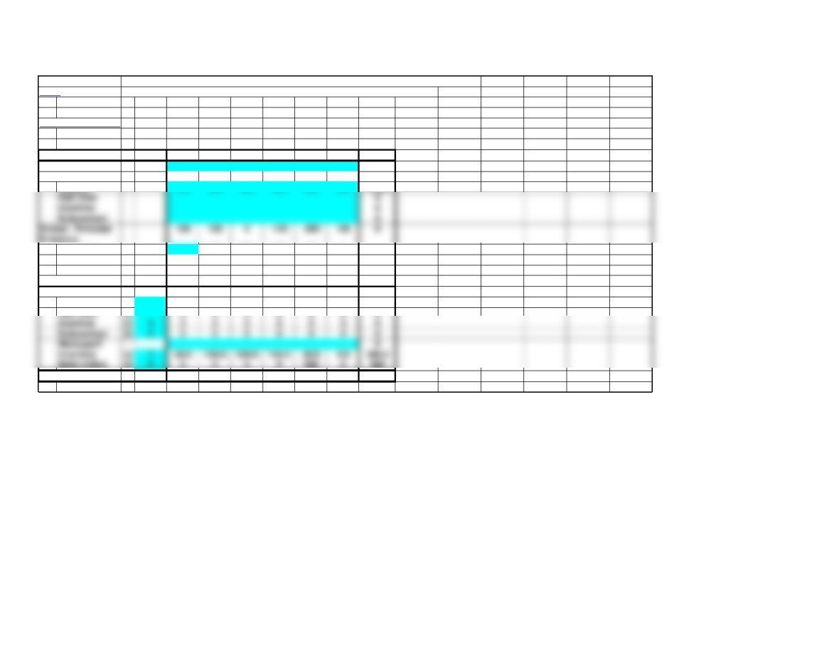
Master Scheduling
Master Scheduling Basic
<Back
Week 0 1 2 3 4 5 6 7 8
Forecast 70 70 70 70
Basic Template: You can simply copy the basic template below and paste into another worksheet.
^Top
Master Scheduling
Week 0 1 2 3 4 5 6 7 8
Forecast 70 70 70 70
Clear
Page 6
Lecture Suggestions – Chapter 13
<Back
Example 2: Aggregate Planning
1. Select the Example 2 worksheet
3. Use spinner button to set number of periods = 6.
4. Enter the following costs per unit: Regular @ 2, Overtime @ 3, Inventory @ 1 Backorders @ 5.
5. Enter forecast for each period in row 5: 200, 200, 300, 400, 500, 200
6. Enter the regular output for each period in column 7: 280, 280, 280, 280, 280, 280. Note that the
7. Point out that Output-Forecast (row 11) shows excess production in periods 1, 2, and 6 but
8. Enter overtime production in row 9, since the maximum overtime is 40, it is optimal to schedule
9. Trace the buildup of inventory in periods 1, 2, and 3 and the depletion of inventory in periods 4 and 5.
10. Also point out that there is a backorder of 80 units from period 5 which made up in period 6 at a cost
of 400 (row 24).
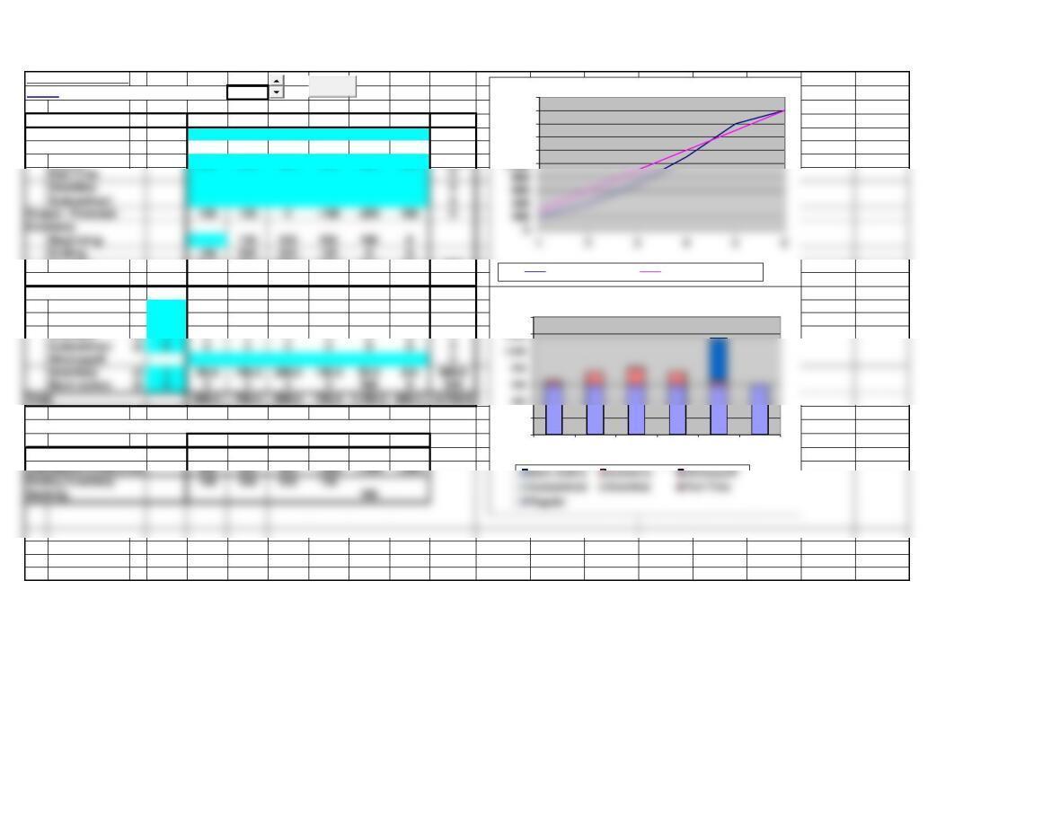
11. Point out in the graph in the lower right hand corner allocation of the various costs by period.
12. Finally, you may want to shift the overtime production, either 1 period earlier or 1 period later and
show that the total cost will be higher in either case.
2. Clear worksheet (press Clear and confirm with OK).
Example 1
Aggregate Planning
<Back Number of periods: 6
Period 1 2 3 4 5 6 Total
Forecast 200 200 300 400 500 200 1,800
Output
Regular 300 300 300 300 300 300 1,800
Average 50.0 150.0 200.0 150.0 50.0 0.0 600
Backlog 0 0 0 0 100 0100
Costs:
Regular @ 2 600 600 600 600 600 600 3,600
Part Time @ 0 0 0 0 0 0 0
Overtime @ 3 0 0 0 0 0 0 0
Subcontract @ 6 0 0 0 0 0 0 0
Hire/Layoff 0
Inventory @ 1 50.0 150.0 200.0 150.0 50.0 0.0 600.0
See the Aggregate Planning tutorial for a demonstration of this template.
1 2 3 4 5 6
Cumulative Forecast 200 400 700 1,100 1,600 1,800
Cumulative Production
Ending Inventory 100 200 200 100
0
200
1,200
1,400
1 2 3 4 5 6
Aggregate Planning – Costs
1,000
1,200
1,400
1,600
1,800
2,000
Cum Forecast Cum Production
Clear
Page 8
Part Time 0
Output – Forecast 100 100 0-100 -200 100 0
Inventory
Example 2
Aggregate Planning
<Back Number of periods: 6
Period 1 2 3 4 5 6 Total
Forecast 200 200 300 400 500 200 1,800
Output
Backlog 0 0 0 0 80 080
Costs:
Regular @ 2 560 560 560 560 560 560 3,360
Part Time @ 0 0 0 0 0 0 0
Overtime @ 3 0 0 120 120 120 0360
Subcontract @ 6 0 0 0 0 0 0 0
Hire/Layoff 0
See the Aggregate Planning tutorial for a demonstration of this template.
1 2 3 4 5 6
Cumulative Forecast 200 400 700 1,100 1,600 1,800
Cumulative Production
Ending Inventory 80 160 180 100
0
200
1,200
1 2 3 4 5 6
Aggregate Planning – Costs
1,200
1,400
1,600
1,800
2,000
Cum Forecast Cum Production
Clear
Page 9
Part Time 0
Output – Forecast 80 80 20 -80 -180 80 0
Inventory
Transportation Model (Basic) Notes Use Solver on Data Ribbon to solve – see notes below.
<Back Do not change or delete unshaded cells.
Input Matrix: Demand for: Period 1 Period 2 Period 3
Beginning Inventory 0 1 2 100
Regular Time 60 61 62 500
Overtime 80 81 82 50
Subcontract 90 91 92 120
Solution Matrix: Total Demand = 2000
Demand for: Period 1 Period 2 Period 3 0
Beginning Inventory 100 0 0 100
Regular Time 400 0100 500
Overtime 50 0 0 50
Subcontract 0 30 030
Regular Time 0 500 0500
Regular Time 0 0 500 500
Period 2
Period 3
Notes: See the Transportation tutorial for a demonstration of a similar template.
Unneeded rows and columns have been hidden in the above template.
1. Enter the problem into the Input Matrix (top shaded area):
Enter the names of periods in the top row (optional).
Supply Used
Period 1
Supply Available
Period 1
Regular Time 63 60 61 500
Overtime 83 80 81 50
Subcontract 93 90 91 120
Regular Time 66 63 60 500
Overtime 86 83 80 50
Subcontract 96 93 90 100
Period 2
Period 3
2. You can manually create solutions in the Solution Matrix (bottom shaded area):
Enter amounts in the row produced and column used in the middle of the Solution Matrix (shaded yellow).
3. Using Solver to find the optimal solution:
Select the Data ribbon, the Solver Add-in must be available in the Analysis group (see note below to add-in Solver).
More… 4. Notes on the Solver solution:
Small numbers in scientific notation (e.g. 2.4091E-11) reflect the precision of Solver and can be treated as zero.
If total demand exceeds total supply then problem is not feasible and you will get an error message.
5. How to Add-In Solver if it does not appear in the Analysis group of the Data ribbon:
Select File (left-most item in main menu at top of screen).
Select Options (left side of dialog box).
Solved Problem 1
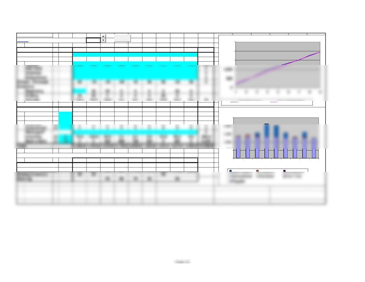
Aggregate Planning
<Back Number of periods: 9
Period 1 2 3 4 5 6 7 8 9 Total
Forecast 190 230 260 280 210 170 160 260 180 1,940
Output
Backlog 0 0 20 80 70 30 030 0230
Costs:
Regular @ 6 1,320 1,320 1,320 1,320 1,320 1,260 1,260 1,260 1,260 11,640
Part Time @ 0 0 0 0 0 0 0 0 0 0
Hire/Layoff 0
See the Aggregate Planning tutorial for a demonstration of this template.
1 2 3 4 5 6 7 8 9
Cumulative Forecast 190 420 680 960 1,170 1,340 1,500 1,760 1,940
Cumulative Production
220 440 660 880 1,100 1,310 1,520 1,730 1,940
Ending Inventory 30 20 20
0
500
2,500
123456789
Aggregate Planning – Costs
1,500
2,000
2,500
Cum Forecast Cum Production
Clear
Part Time 0
Output – Forecast 30 -10 -40 -60 10 40 50 -50 30 0
Inventory
Solved Problem 2
Aggregate Planning
<Back Number of periods: 8
Period 1 2 3 4 5 6 7 8 9 10 11 12 Total
Forecast 1,200 1,200 1,400 3,000 1,200 1,200 1,200 1,200 11,600
Output
Output – Forecast 0 0 -200 200 000000000
Inventory
Beginning 0 0 0 0 0 0 0 0 0 0 0
Ending 0 0 0 0 0 0 0 0 0 0 0 0
Costs:
Regular @ 4 4,800 4,800 4,800 4,800 4,800 4,800 4,800 4,800 0 0 0 0 38,400
Part Time @ 5 0 0 0 10,000 0 0 0 0 0 0 0 0 10,000
Overtime @ 0 0 0 0 0 0 0 0 0 0 0 0 0
Subcontract @ 0 0 0 0 0 0 0 0 0 0 0 0 0
Hire/Layoff 100 100
Total 4,800.0 4,800.0 5,100.0 14,800.0 4,800.0 4,800.0 4,800.0 4,800.0 0.0 0.0 0.0 0.0 48,700.0
See the Aggregate Planning tutorial for a demonstration of this template.
12345678910 11 12
Cumulative Forecast 1,200 2,400 3,800 6,800 8,000 9,200 10,400 11,600 11,600 11,600 11,600 11,600
Cumulative Production 1,200 2,400 3,600 6,800 8,000 9,200 10,400 11,600 11,600 11,600 11,600 11,600
Ending Inventory
0
2,000
4,000
14,000
16,000
1 2 3 4 5 6 7 8 9 10 11 12
Aggregate Planning – Costs
0
2,000
8,000
10,000
12,000
14,000
1 2 3 4 5 6 7 8 9 10 11 12
Clear
Page 13
Part Time 2,000 2,000