11 – 1
Chapter 11
Integer Linear Programming
Case Problem 1: Textbook Publishing
An integer programming model can be used advantageously to assist in developing recommendations.
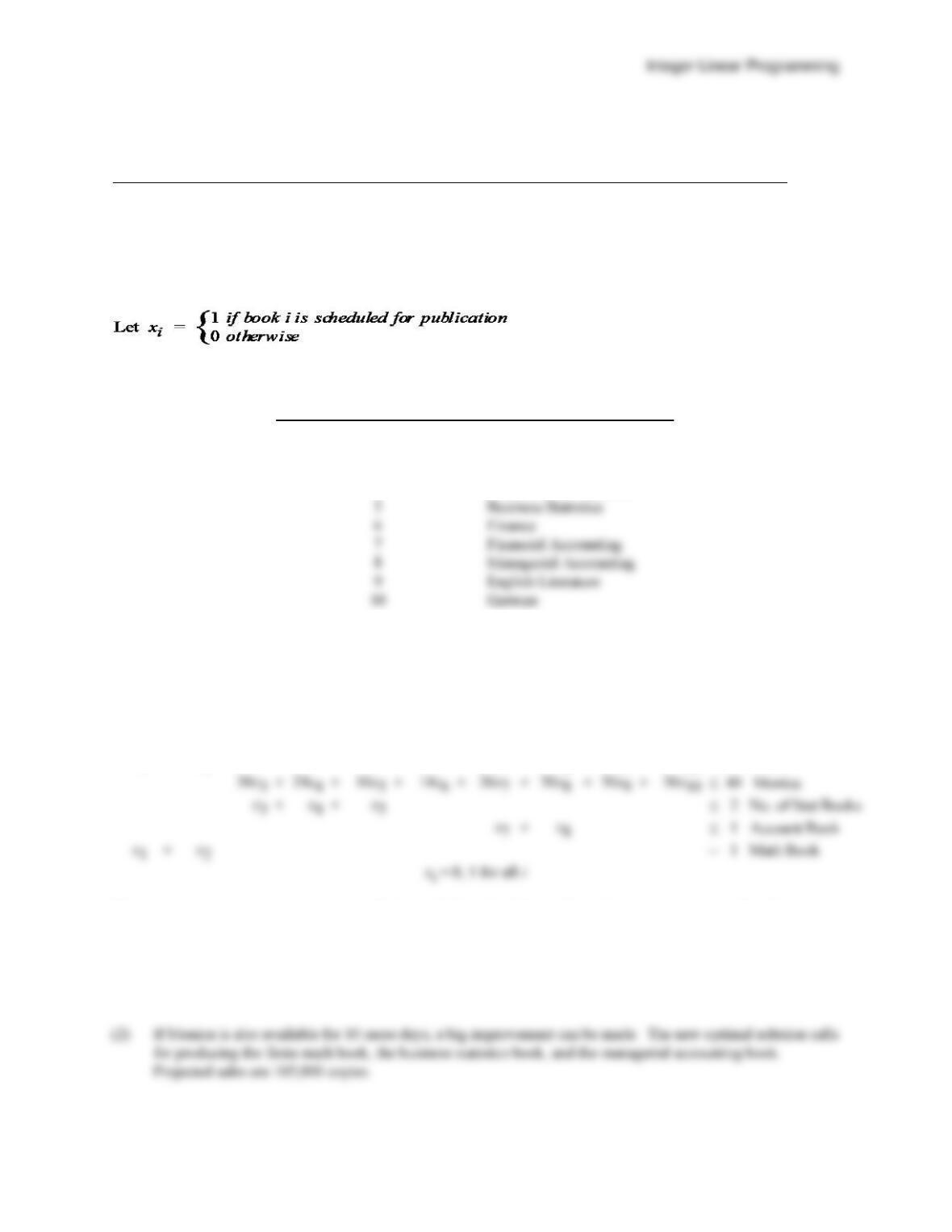
The subscripts correspond to the books as follows:
i
Book
1
Business Calculus
2
Finite Math
3
General Statistics
4
Mathematical Statistics
5
Business Statistics
6
7
Financial Accounting
8
Managerial Accounting
9
English Literature
An integer programming model for maximizing projected sales (thousands of units) subject to the restrictions
mentioned is given.
Max
20x1
+
30x2
+
15x3
+
10x4
+
25x5
+
18x6
+
25x7
+
50x8
+
20x9
+
30x10
s.t.
30x1
+
16x2
+
24x3
+
20x4
+
10x5
+
40x9
60 John
40x1
+
24x2
+
24x7
+
28x8
+
34x9
+
50x10
40 Susan
30x3
+
24x4
+
16x5
+
14x6
+
26x7
+
30x8
+
30x9
+
36x10
40 Monica
+
+
2 No. of Stat Books
+
1 Account Book
+
=
1 Math Book
The optimal solution (x2 = x5 = x6 = 1) calls for publishing the finite math, the business statistics and the finance
books. Projected sales are 73,000 copies.
(1) If Susan can be made available for another 12 days, the optimal solution is x2 = x8 = 1. This calls for
publishing the finite math and managerial accounting texts for projected sales of 80,000 copies.
Chapter 11
11 –
2
(3) The solution in (2) above does not include any new books. In the long run this would appear to be a bad
strategy for the company. A variety of modifications can be made to the model to examine the short run
impact of postponing a revision. For instance, a constraint could be added to require publication of at least
one new book.
Case Problem 2: Yeager National Bank
A mixed integer linear programming (MILP) model can be used advantageously to assist in preparing a report for
Mr. Wolff. Since the annual fixed costs of operating the lockboxes are not known exactly we formulate a model that
We use the following variable definitions:
P = 1 if a lockbox is in Phoenix; 0 otherwise
S = 1 if a lockbox is in Salt Lake City; 0 otherwise
A = 1 if a lockbox is in Atlanta; 0 otherwise
B = 1 if a lockbox is in Boston; 0 otherwise
The MILP model has 24 variables and 26 constraints. The objective function calls for minimizing lost interest
income. To see how the objective function coefficients are computed, consider assigning the Northwest region to
Phoenix. Daily collections are $80,000 and it takes 4 days to receive and process payments. At a 15% rate Yeager
could save $48,000 = (.15)(4)($80,000) annually over this assignment if the Northwest collections could be credited
to their account instantaneously. A similar calculation is made for all the other potential assignments. The
objective function coefficients for P, S, A, and B are zero since we are not including the cost of operating the
lockboxes at this stage.
Integer Linear Programming
11 –
3
INTEGER LINEAR PROGRAMMING PROBLEM
MIN
48PNW+27PSW+112.5PCE+135PNE+60PSE+24SNW+40.5SSW+67.5SCE+108SNE+90SSE+48ANW+5
4ASW+67.5ACE+81ANE+30ASE+48BNW+81BSW+90BCE+54BNE+45BSE
S.T.
1) 1PNW+1SNW+1ANW+1BNW=1
2) +1PSW+1SSW+1ASW+1BSW=1
9) +1PNE–1P<0
10) +1PSE–1P<0
11) +1SNW–1S<0
12) +1SSW–1S<0
13) +1SCE–1S<0
14) +1SNE–1S<0
21) +1BNW–1B<0
22) +1BSW–1B<0
23) +1BCE–1B<0
24) +1BNE–1B<0
OPTIMAL SOLUTION
Objective Function Value = 231.000
Variable Value
————– —————
PNW 0.000
PSW 0.000
SNW 1.000
SSW 1.000
SCE 1.000
SNE 0.000
Chapter 11
11 –
4
ASE 0.000
BNW 0.000
BSW 0.000
BCE 0.000
Constraint Slack/Surplus
————– —————
1 0.000
2 0.000
3 0.000
8 0.000
9 0.000
10 0.000
11 0.000
12 0.000
17 0.000
18 0.000
19 0.000
20 0.000
21 1.000
With 2 lockbox locations, the lost interest income is $231,000. Resolving with values of 1, 3, and 4 on the right-
hand-side of constraint 26 provides the following:
No. of
Lockboxes
Locations
Lost Interest
Income ($)
1
Atlanta
280,500
2
Salt Lake City & Boston
231,000
3
Salt Lake City, Atlanta & Boston
216,000
4
Salt Lake City, Phoenix, Atlanta & Boston
202,500
11 –
5
Case Problem 3: Production Scheduling with Changeover Costs
A mixed integer programming model can be used advantageously to assist in developing recommendations. We
describe such a model here; it has 48 decision variables and 64 constraints. We show here how to use Microsoft
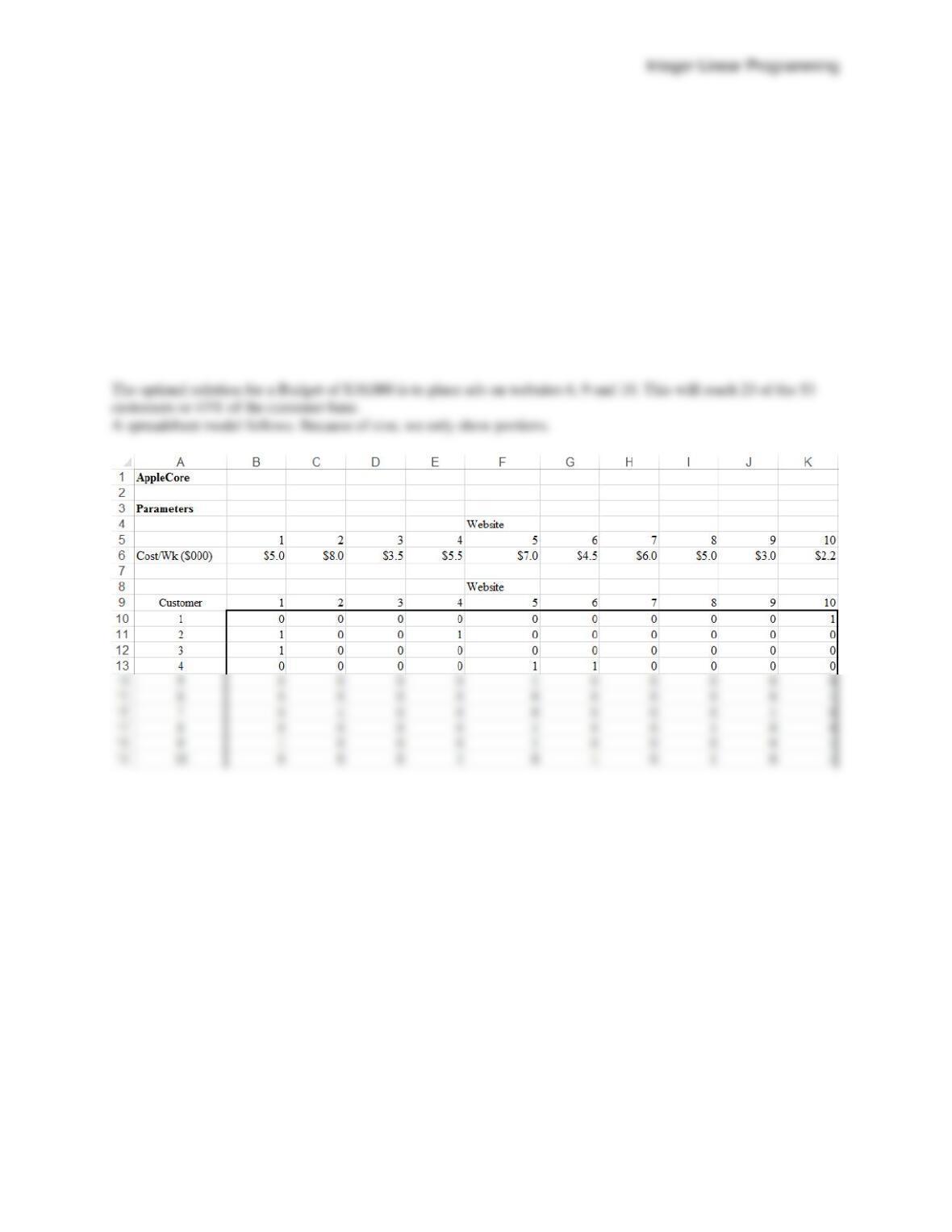
Excel to formulate and solve the problem. The spreadsheet at the end shows how we set up the problem and the
optimal solution. We describe the model now.
Variables
There are variables for production, inventory, setup, and changeover in each week.
Pi = number of P-Heads produced in week i
Hi = number of H-Heads produced in week i
Constraints
There are constraints for production capacity, inventory balance, maintenance of safety stock, and enforcement of
changeovers. Also, Excel requires that you identify the 0-1 (binary) variables in the Solver dialog box. The
constraints as specified in the Excel Solver dialog box are as follows (references are to cells of the spreadsheet):
B20:C27 B34:C41 production capacity, or nonnegativity of slack
G20:G27 H34:H41 forces Changei to 1 when a changeover occurs
G20:G27 I34:I41
Note that even though the Changei variable must also be integer it is not necessary to require it because
minimization will never let it be any bigger than it has to be. And, the second set of constraints force it to be 1
whenever the setup variable changes from 1 to 0 or from 0 to 1.
Objective
We want to minimize total cost which is represented by cell J23 in the spreadsheet. It is the sum of production cost,
inventory cost, and changeover cost.
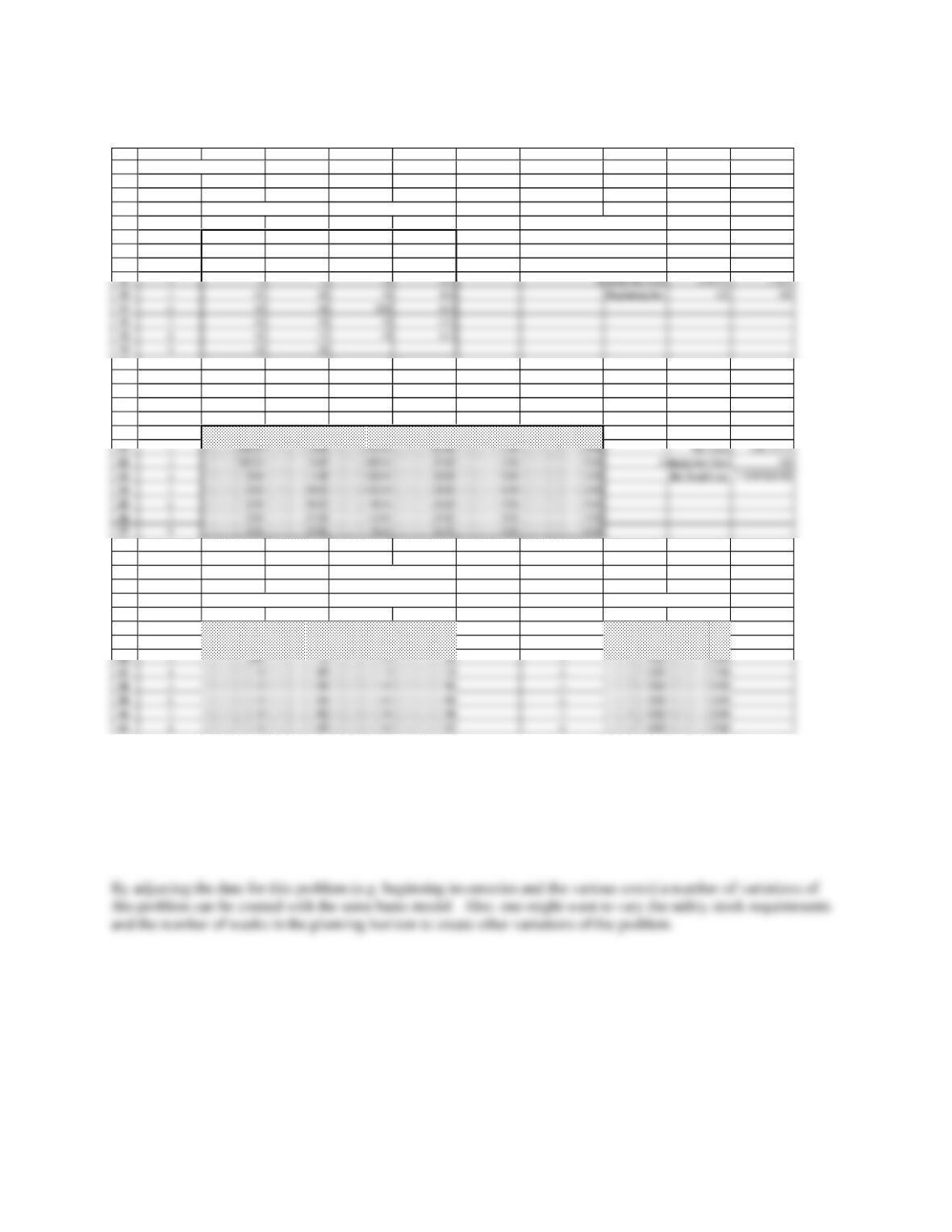
The Spreadsheet
Chapter 11
11 –
6
The spreadsheet formulation and solution are shown.
Solution Comments
The spreadsheet contains the optimal solution. The minimum total cost is $119,154.35. The components of that
cost are production: $117,374, inventory: $1280.35 and changeover: $500. From cells F20:F27 we see that the line
will be setup to produce P-Heads in weeks 1-3 and H-Heads in weeks 4-8. Cell G23 shows that there will be a
changeover from producing P-Heads to H-Heads at the beginning of week 4.
1
2
3
4
5
6
7
8
15
16
17
18
19
20
28
29
30
31
32
33
34
35
A B C D E F G H I J
Production Sche duling
Product Demand Safety S tock P H
Week P H P H Production Cos t 225 310
155 38 44 30.4 Max Weekly Rate 100 80
255 38 35.2 24 Changeover Cos t 500 500
344 30 0 0 Weekly Inv. Rate 0.00375 0.00375
Mode l
Week P H Inv. P Inv. H Setup P Changeover
1 18.00 0.00 88.00 105.00 1.00 0.00 Prod. Cost 117374
Inventory Balance
Beginning Inv. + Prod.
Production Capacity – Ending Inv. Changeover Def.
Week P HP HWeek To P if 1 To H if 1
1 100 0 55 38 1 0.00 0.00
2 100 0 55 38 2 0.00 0.00
11 –
7
Case Problem4: Applecore Children’s Clothing
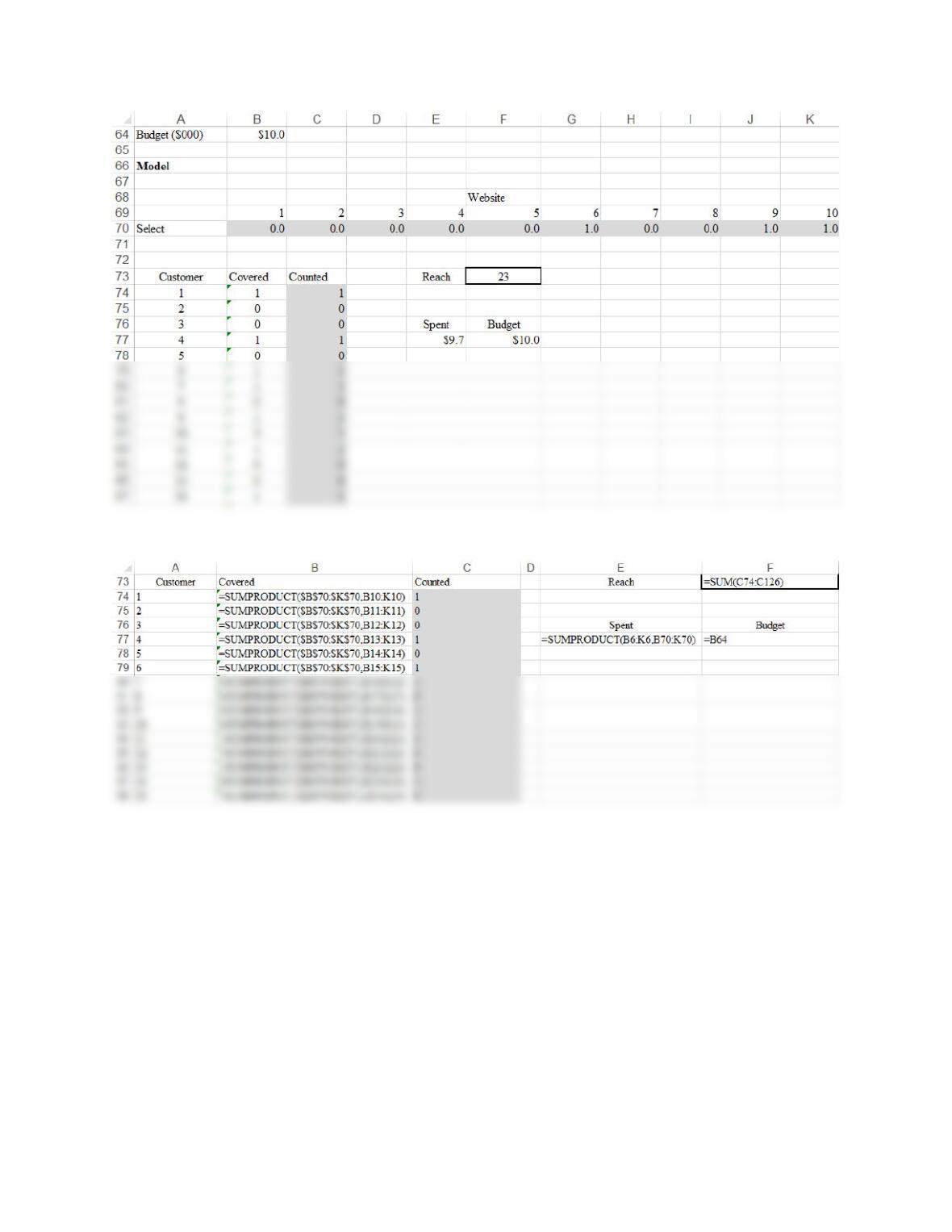
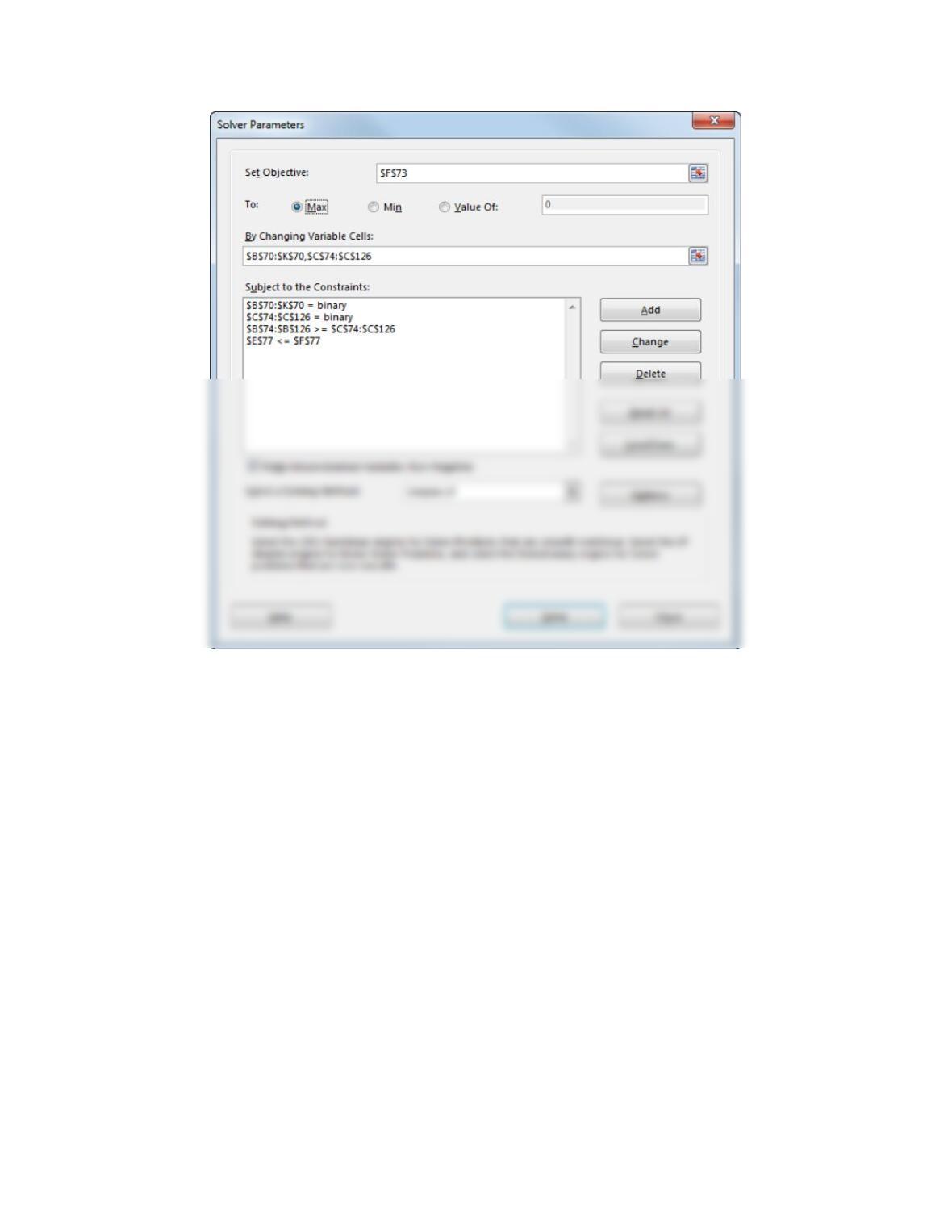
The Model:
Let yi = 1 if customer i is reached, 0 if not, i=1,2,…53
xj = 1 if we place an ad on website j, j=1,2,..10
Max y1 + Y2 + Y3 + … + Y53
s.t
x10 ≥ y1
x2 + x4 ≥ y2
x1 ≥ y3
● ● ●
● ● ●
x2 + x5 + x8 + x9 + x10 ≥ y53
5×1 + 8×2 + 3.5×3 + 5.5×4 + 7.0×5 + 4.5×6 + 6.0×7 + 5.0×8 + 3.0×9 + 2.2×10 ≤ 10
Chapter 11
11 –
8
Integer Linear Programming
11 –
9
Chapter 11
11 –
10
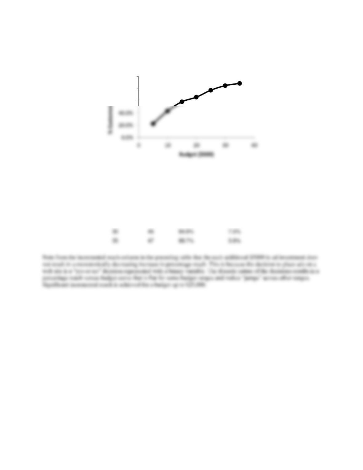
We solve the model for various budget levels:
Budget
Reach
% Reach
Incremental Reach
5
12
22.6%
10
23
43.4%
20.8%
15
31
58.5%
15.1%
20
35
66.0%
7.5%
25
41
77.4%
11.3%
30
45
84.9%
60.0%
80.0%
100.0%