
Copyright © 2012 by The McGraw Hill Companies, Inc. All rights reserved.
Supplement to Chapter Ten – Acceptance Sampling
Templates: Acceptance Sampling (B)
Lecture Suggestions
(B) – includes Basic template
Example 2
See Instructions template for complete instructions.
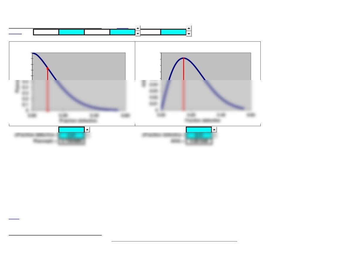
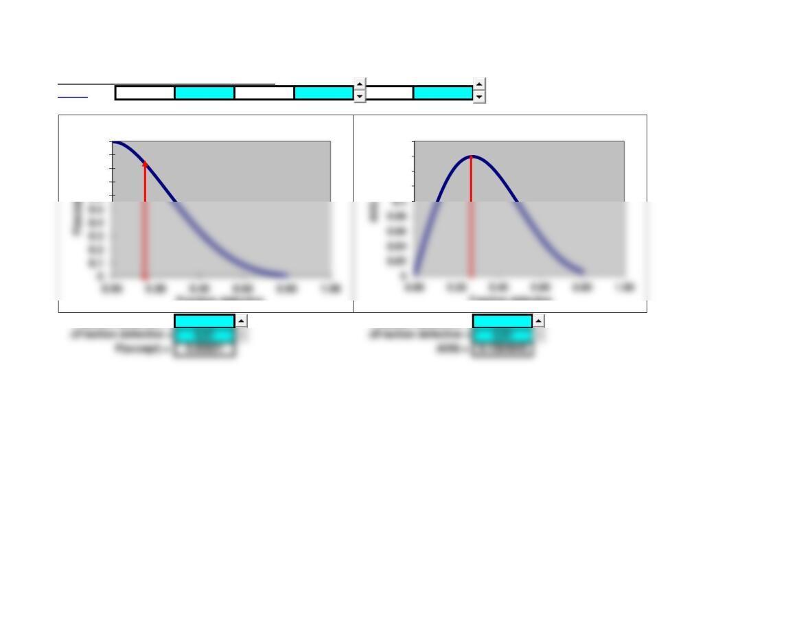
Acceptance Sampling
Acceptance Sampling – Binomial Distribution Basic
<Back N = 500 n = 10 c = 1
Fraction defective = 0.1 Fraction defective = 0.15
Basic Template: You can simply copy the basic template below and paste into another worksheet.
^Top If you also copy the graphs you will have to fix the cell references in the graph
(right-click on the graph, click Select Data…, and Edit the Series values for each series).
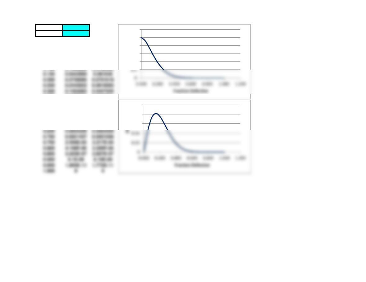
Acceptance Sampling – Binomial Distribution
0.7361
0.6
0.7
0.8
0.9
1
Operating Characteristic Curve
0.0816
0.05
0.06
0.07
0.08
0.09
Average Outgoing Quality
Page 2
Acceptance Sampling
n = 10
c = 1
Fraction
Defective P(Accept) AOQ
0.000 1 0
0.050 0.9138616 0.0456931
0.350 0.0859544 0.0300841
0.400 0.0463574 0.018543
0.450 0.0232571 0.0104657
0.500 0.0107422 0.0053711
0.550 0.0045022 0.0024762
0.600 0.0016777 0.0010066
0.650 0.0005399 0.0003509
0.700 0.0001437 0.0001006
1.000 0 0
0.4
0.6
0.8
1
1.2
P(accept)
0.06
0.08
0.1
Page 3
0.100 0.7360989 0.0736099
0.150 0.5442998 0.081645
0.200 0.3758096 0.0751619
0.300 0.1493083 0.0447925
Acceptance Sampling
0 1
0.0000 1 -1.32E-16 1.87E-11 0.95
0.0275 0.970615 0.026692 9.1E-09 0.9
0.0825 0.802837 0.066234 4.2E-06 0.8
0.1375 0.59101 0.081264 0.000144 0.7
0.1925 0.398881 0.076785 0.001678 0.6
0.2200 0.318469 0.070063 0.004502 0.55
0.2475 0.249704 0.061802 0.010742 0.5
0.3025 0.145456 0.044001 0.046357 0.4
0.3575 0.078689 0.028131 0.149308 0.3
0.4125 0.039294 0.016209 0.37581 0.2
0.4400 0.026864 0.01182 0.5443 0.15
0.4675 0.017927 0.008381 0.736099 0.1
0.4950 0.011652 0.005768 0.913862 0.05
0.5225 0.007359 0.003845 1 0
0.1 0
0.1 0.736099
0.15 0 0
0.15 0.5443 0.081645
Lecture Suggestions – Supplement to Chapter 10
<Back
Example 1: Acceptance Sampling
1. Select the Example 1.
2. Enter the following data: N=5000, n=80, and c=2
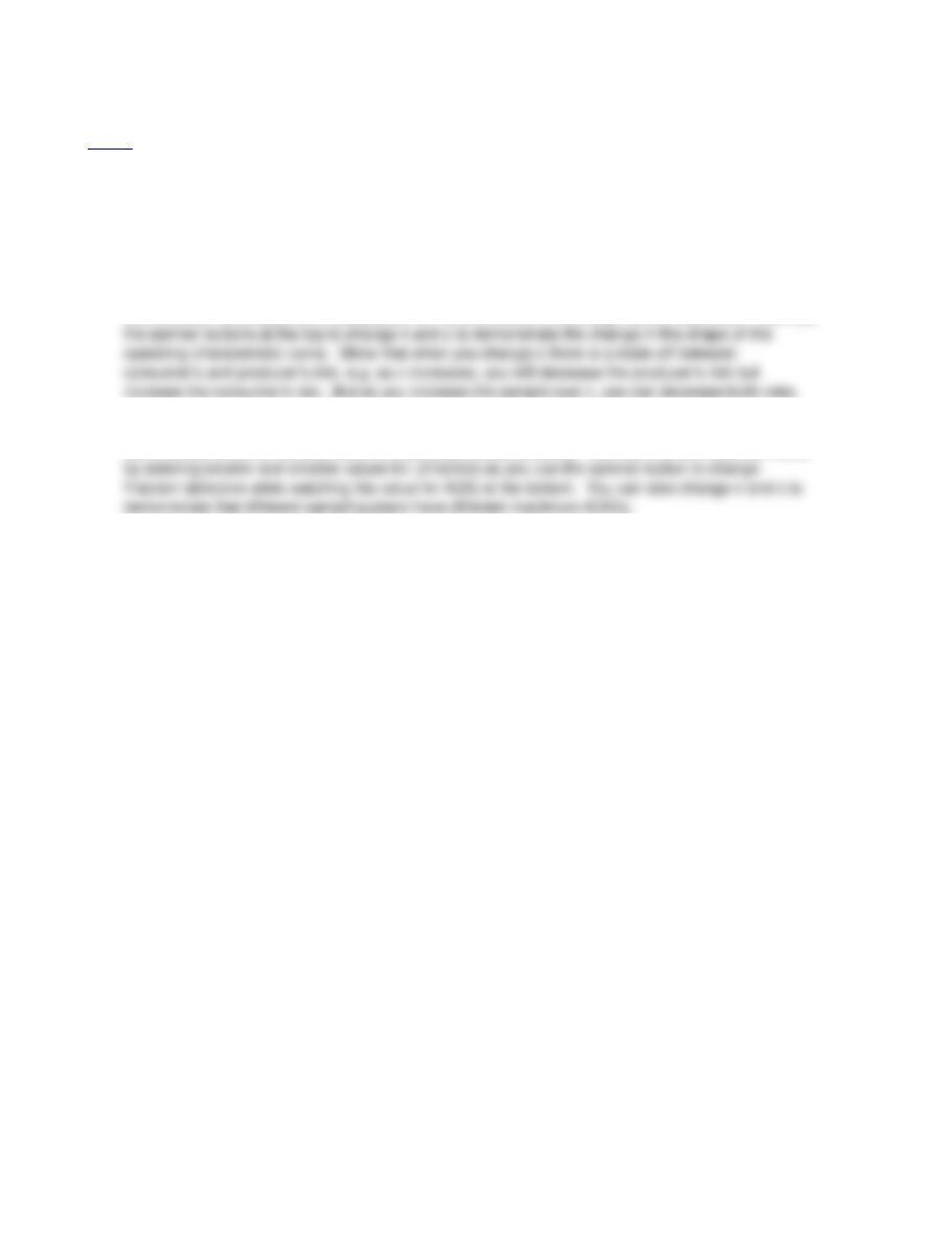
3. The operating characteristic curve is on the left. Use the spinner button below the graph to
demonstrate the probability of acceptance for various levels of incoming fraction defectives. Also use
4. The average outgoing quality curve is on the right. Use the spinner button below the graph to
demonstrate AOQ for various levels of incoming fraction defective. You can find the maximum AOQ
Example 1
Acceptance Sampling – Binomial Distribution
<Back N = 5000 n = 80 c = 2
Fraction defective = 0.01 Fraction defective = 0.03
Note: Example 1 in text uses Poisson approximation to the Binomial.
0.9534
0
0.1
0.2
0.3
0.5
0.7
0.9
1
0.00 0.05 0.10 0.15 0.20
Fraction defective
Operating Characteristic Curve
0.0170
0
0.004
0.01
0.014
0.016
0.018
0.00 0.05 0.10 0.15 0.20
Fraction defective
Average Outgoing Quality
Page 6
Example 1
0 1
0.0000 1 -2.26E-17 9.4E-99 0.95
0.0075 0.977405 0.007331 2.57E-75 0.9
0.0225 0.731247 0.016453 6.15E-52 0.8
0.0375 0.418904 0.015709 2.57E-38 0.7
0.0525 0.202443 0.010628 1.06E-28 0.6
0.0600 0.134446 0.008067 8.71E-25 0.55
0.0675 0.08713 0.005881 2.68E-21 0.5
0.0825 0.034409 0.002839 2.61E-15 0.4
0.0975 0.01269 0.001237 2.5E-10 0.3
0.1050 0.007538 0.000791 3.83E-08 0.25
0.1125 0.004419 0.000497 3.86E-06 0.2
0.1275 0.001463 0.000187 0.010684 0.1
0.1425 0.000463 6.6E-05 1 0
0.1500 0.000256 3.84E-05
0.01 0
0.01 0.953447
0.03 0 0
0.03 0.568123 0.017044
Page 7
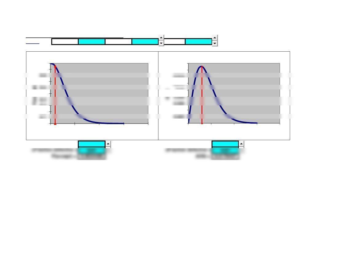
Example 2
Acceptance Sampling – Binomial Distribution
<Back N = 500 n = 10 c = 1
Fraction defective = 0.1 Fraction defective = 0.15
0.7361
0
0.1
0.2
0.4
0.7
0.8
1
0.00 0.20 0.40 0.60
P(accept)
Fraction defective
Operating Characteristic Curve
0
0.03
0.04
0.07
0.09
0.00 0.20 0.40 0.60
AOQ
Fraction defective
Average Outgoing Quality
Page 8
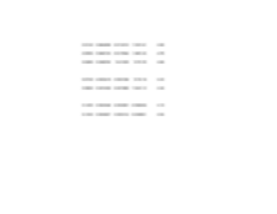
Example 2
0 1
0.0000 1 -1.32E-16 1.87E-11 0.95
0.0275 0.970615 0.026692 9.1E-09 0.9
0.0825 0.802837 0.066234 4.2E-06 0.8
0.1375 0.59101 0.081264 0.000144 0.7
0.1650 0.490348 0.080907 0.00054 0.65
0.1925 0.398881 0.076785 0.001678 0.6
0.2200 0.318469 0.070063 0.004502 0.55
0.2475 0.249704 0.061802 0.010742 0.5
0.3025 0.145456 0.044001 0.046357 0.4
0.3575 0.078689 0.028131 0.149308 0.3
0.4125 0.039294 0.016209 0.37581 0.2
0.4400 0.026864 0.01182 0.5443 0.15
0.4675 0.017927 0.008381 0.736099 0.1
0.4950 0.011652 0.005768 0.913862 0.05
0.5225 0.007359 0.003845 1 0
0.5500 0.004502 0.002476
Page 9
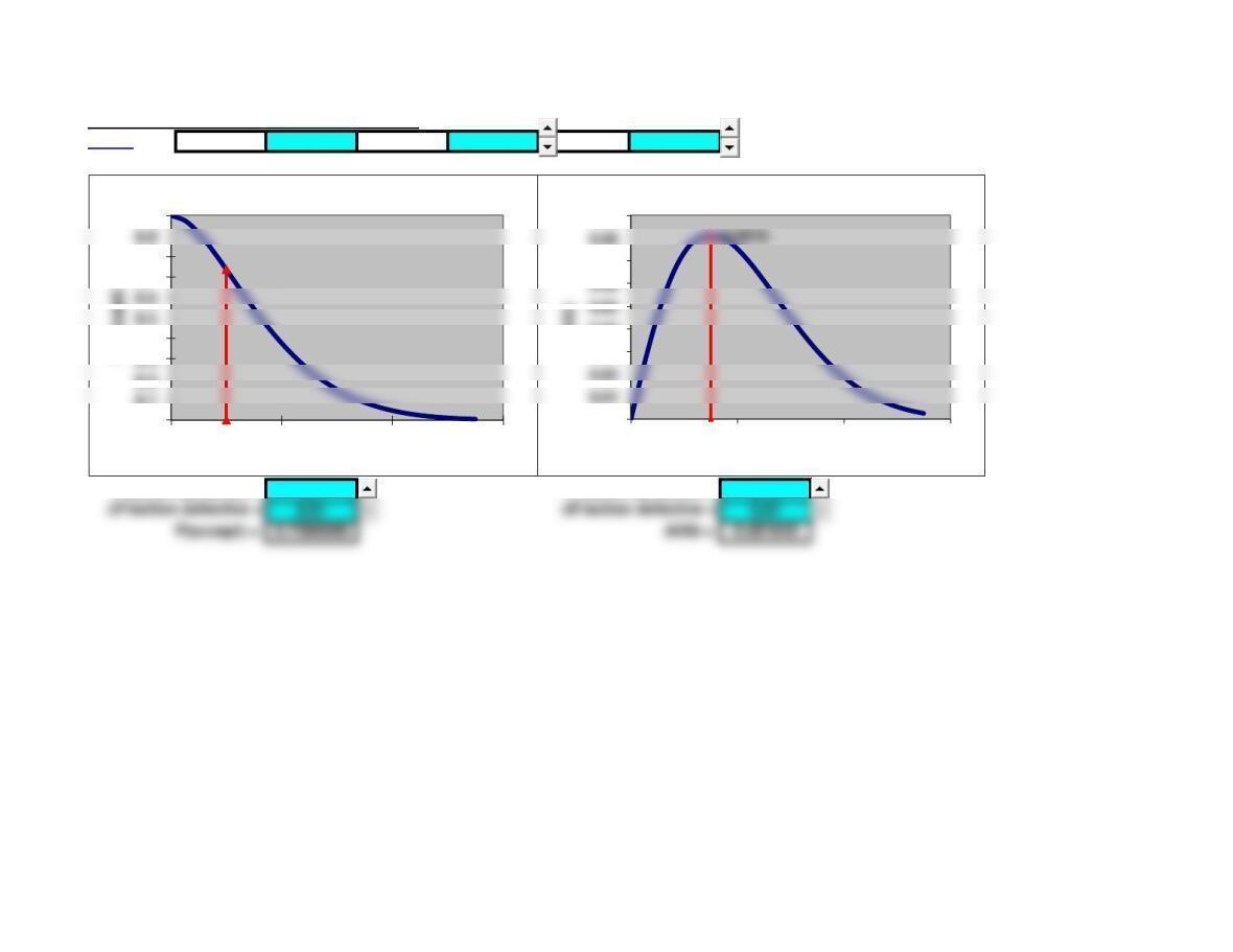
Solved Problem 2
Acceptance Sampling – Binomial Distribution
<Back N = 300 n = 5 c = 1
Fraction defective = 0.15 Fraction defective = 0.27
0.8352
0.6
0.7
0.8
0.9
1
Fraction defective
Operating Characteristic Curve
0.1595
0.12
0.14
0.16
0.18
Fraction defective
Average Outgoing Quality
Page 10
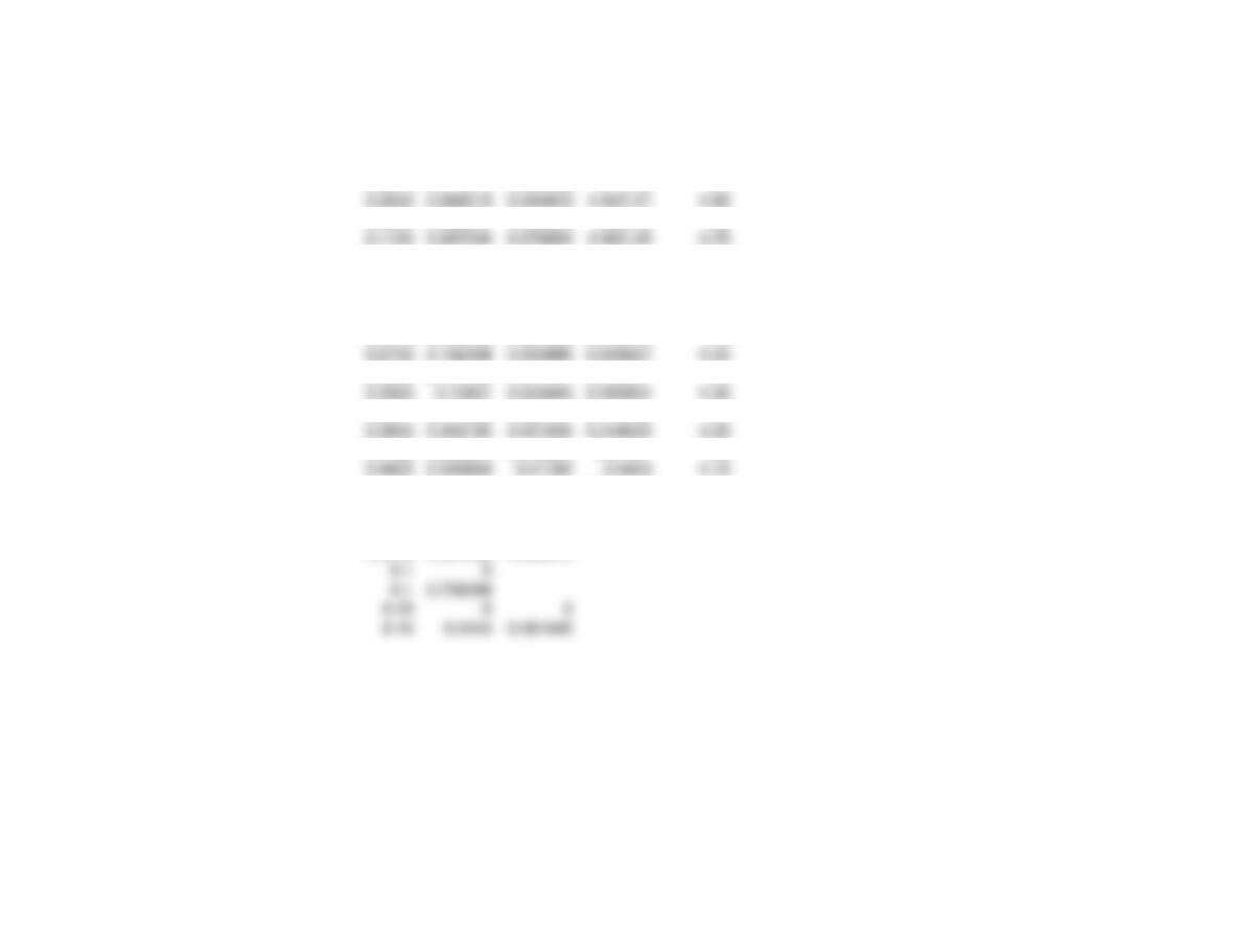
Solved Problem 2
0.1200 0.887549 0.106506 0.00672 0.8
0.1600 0.816509 0.130641 0.015625 0.75
0.2000 0.73728 0.147456 0.03078 0.7
0.3600 0.409364 0.147371 0.1875 0.5
0.4000 0.33696 0.134784 0.256218 0.45
0.4400 0.271432 0.11943 0.33696 0.4
0.5200 0.163499 0.08502 0.52822 0.3
0.6000 0.08704 0.052224 0.73728 0.2
0.6400 0.059794 0.038268 0.83521 0.15
0.6800 0.039007 0.026525 0.91854 0.1
0.7600 0.013404 0.010187 1 0
0.15 0
0.15 0.83521
0.27 0 0
0.27 0.590683 0.159485
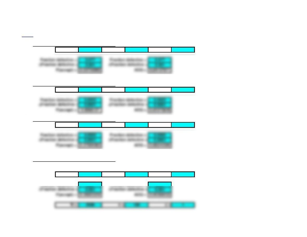
Supplement to Chapter 10 – Problems 2-6 Note: This worksheet displays results only, you must copy the shaded
<Back area into the corresponding template to make additional calculations.
2. Acceptance Sampling – Binomial Distribution
N = 4000 n = 20 c = 1
3a. Acceptance Sampling – Binomial Distribution
N = 8000 n = 15 c = 0
3b-c. Acceptance Sampling – Binomial Distribution
N = 8000 n = 150 c = 0
4. Acceptance Sampling – Binomial Distribution
Note: AOQL is estimated from each of the following sampling plans.
4a.
N = 3000 n = 100 c = 0
N = 3000 n = 100 c = 1
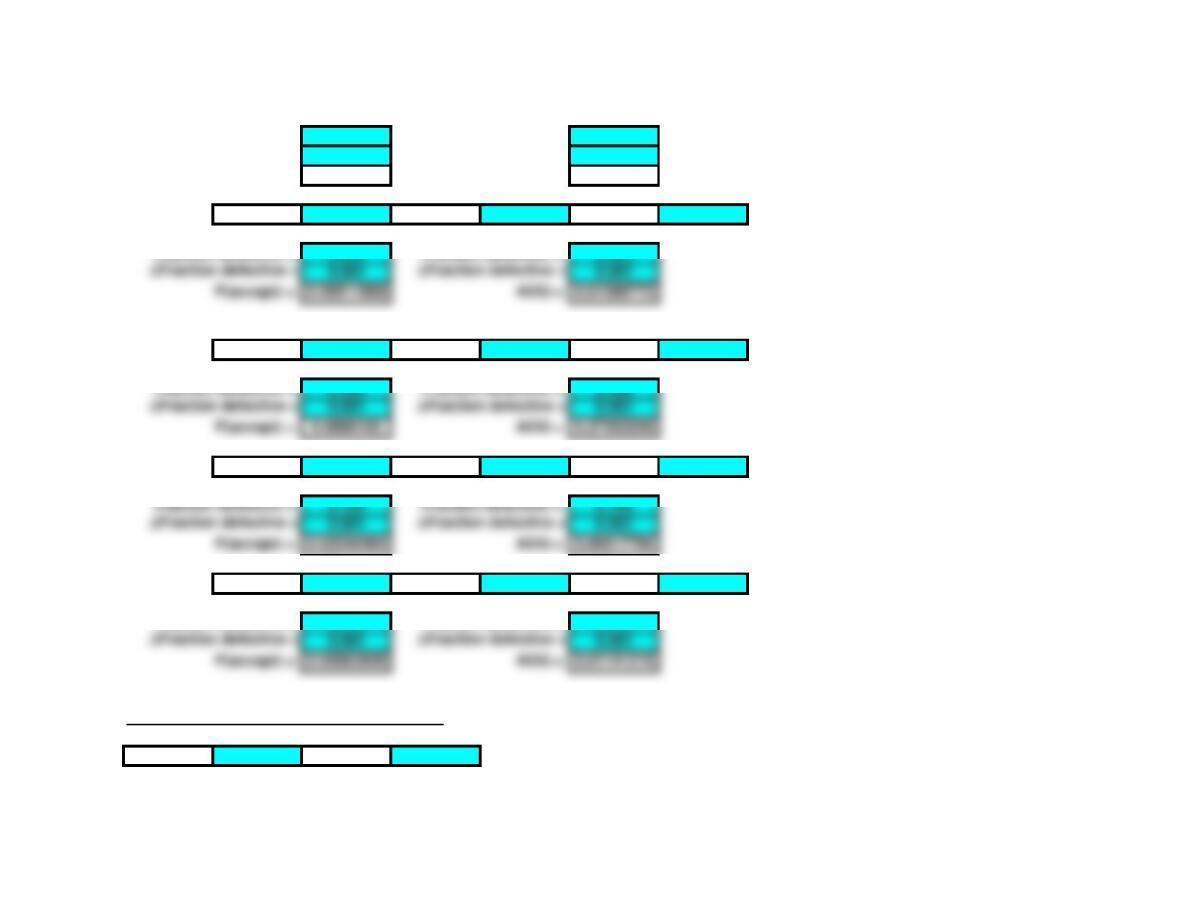
Fraction defective = 0.016 Fraction defective = 0.016
DFraction defective = 0.001 DFraction defective = 0.001
P(accept) = 0.52336811 AOQ = 0.00837389
N = 3000 n = 100 c = 2
Fraction defective = 0.023 Fraction defective = 0.023
4b. N = 3000 n = 5 c = 2
Fraction defective = 0.398 Fraction defective = 0.398
DFraction defective = 0.001 DFraction defective = 0.001
P(accept) = 0.6860102 AOQ = 0.27303206
N = 3000 n = 20 c = 2
Fraction defective = 0.109 Fraction defective = 0.109
DFraction defective = 0.001 DFraction defective = 0.001
P(accept) = 0.62548494 AOQ = 0.06817786
N = 3000 n = 120 c = 2
Fraction defective = 0.019 Fraction defective = 0.019
DFraction defective = 0.001 DFraction defective = 0.001
5c. Acceptance Sampling – Binomial Distribution
n = 15 c = 2
DFraction defective = 0.001 DFraction defective = 0.001
P(accept) = 0.59511868 AOQ = 0.01368773
Fraction defective = 0.05
DFraction defective = 0.01
P(accept) = 0.96379976
5d. Acceptance Sampling – Binomial Distribution
n = 15 c = 2
6c. Acceptance Sampling – Binomial Distribution
n = 15 c = 1
Fraction defective = 0.05 Fraction defective = 0.05
DFraction defective = 0.05 DFraction defective = 0.05
P(accept) = 0.82904746 AOQ = 0.04145237
Fraction defective = 0.1 Fraction defective = 0.1
DFraction defective = 0.05 DFraction defective = 0.05
P(accept) = 0.54904302 AOQ = 0.0549043
Fraction defective = 0.15 Fraction defective = 0.15
DFraction defective = 0.05 DFraction defective = 0.05
P(accept) = 0.31858598 AOQ = 0.0477879
Fraction defective = 0.2 Fraction defective = 0.2
DFraction defective = 0.05 DFraction defective = 0.05
P(accept) = 0.16712577 AOQ = 0.03342515
Fraction defective = 0.2
DFraction defective = 0.01
P(accept) = 0.39802321