Chapter 10 – Quality Control
10–13
15.
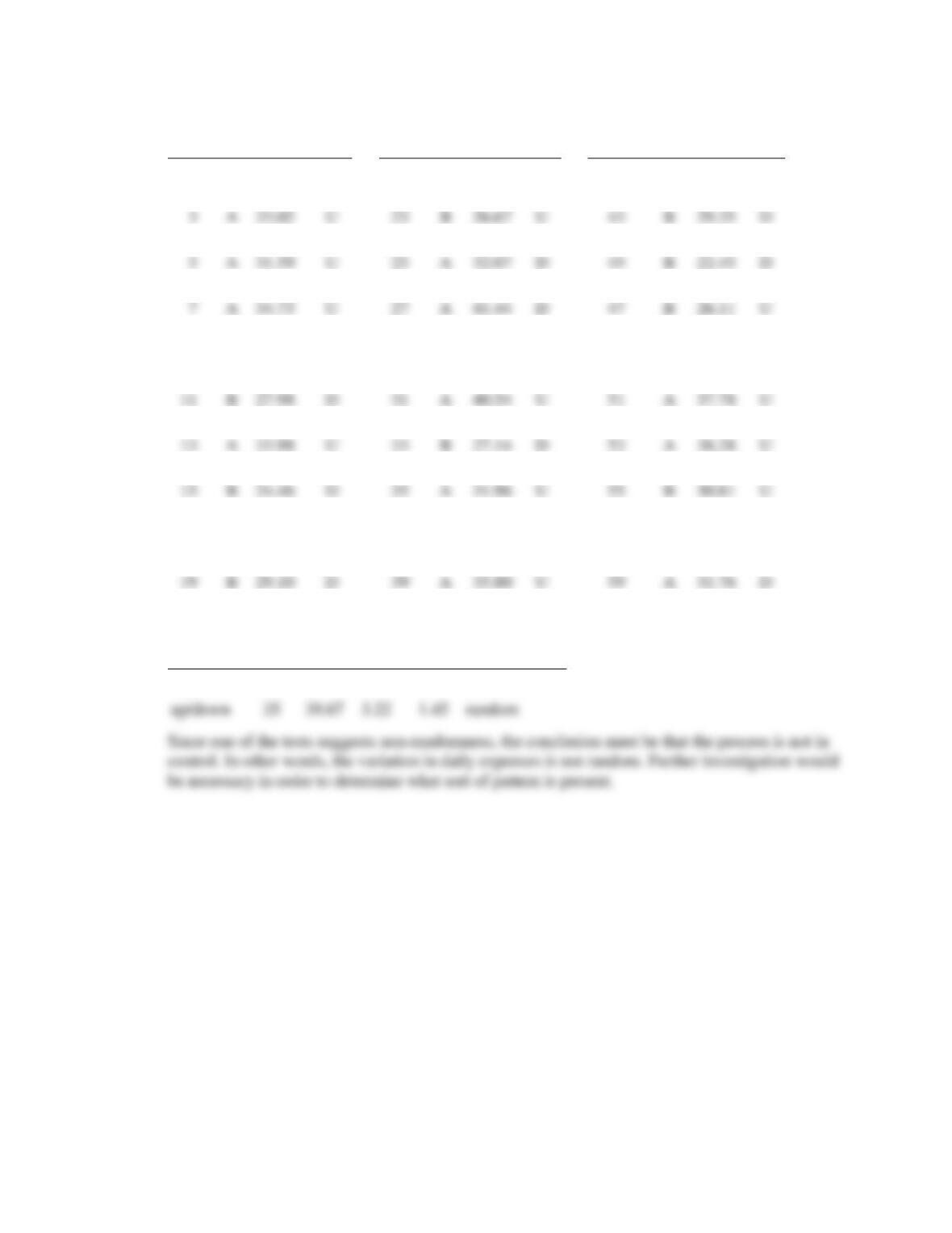
Day
Amount
Day
Amount
Day
Amount
1
B
27.69
−
21
B
28.60
U
41
B
26.76
D
2
B
28.13
U
22
B
20.02
D
42
B
30.51
U
4
B
30.31
D
24
A
36.40
U
44
B
24.09
D
A
31.59
U
25
A
32.07
D
45
B
22.45
D
6
A
33.64
U
26
A
44.10
U
46
B
25.16
U
7
A
34.73
U
27
A
41.44
D
47
B
26.11
U
8
A
35.09
U
28
B
29.62
D
48
B
29.84
U
9
A
33.39
D
29
B
30.12
U
49
A
31.75
U
10
A
32.51
D
30
B
26.39
D
50
B
29.14
D
11
B
27.98
D
31
A
40.54
U
51
A
37.78
U
12
A
31.25
U
32
A
36.31
D
52
A
34.16
D
13
A
33.98
U
33
B
27.14
D
53
A
38.28
U
14
B
25.56
D
34
B
30.38
U
54
B
29.49
D
15
B
24.46
D
35
A
31.96
U
55
B
30.81
U
16
B
29.65
U
36
A
32.03
U
56
B
30.60
D
17
A
31.08
U
37
A
34.40
U
57
A
34.46
U
18
A
33.03
U
38
B
25.67
D
58
A
35.10
U
19
B
29.10
D
39
A
35.80
U
59
A
31.76
D
20
B
25.19
D
40
A
32.23
D
60
A
34.90
U
Summary:
Test
obs.
exp.
z
Conclusion
median
22
31
3.84
–2.34
non-random
up/down
35
39.67
3.22
–1.45
random
3
A
33.02
U
23
B
26.67
U
43
B
29.35
D
Chapter 10 – Quality Control
10–14
16.
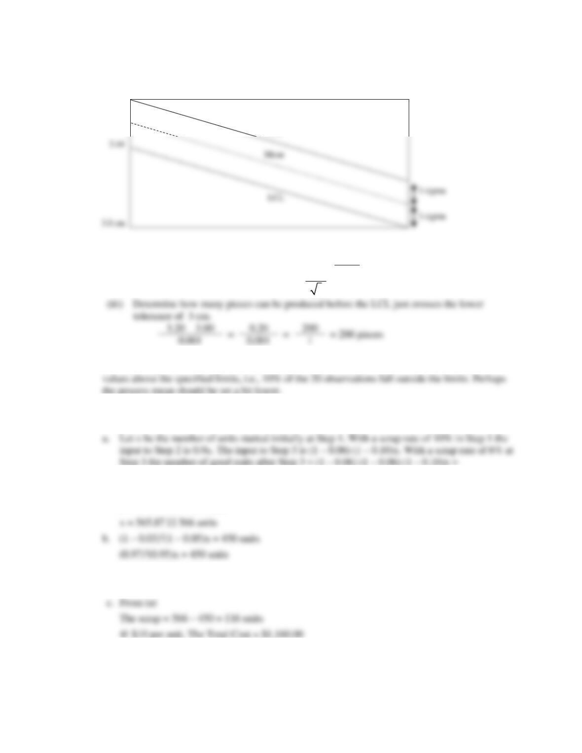
(i)
The upper control limit is 6 standard deviations above the lower control limits.
(ii) When UCL = 3.5 cm, the LCL = 3.5 – 6
0.05 3.5 0.30 3.2 c
1m= − =
17. It is necessary to see if the process variability is within 9.96 and 10.35. Two observations have
18. 1 Step 10% scrap, 2nd 6%, and 3rd 6%.
(0.94)2(0.90)x.
The required output is 450 units
(0.94)2(0.90)x = 450 units
x = 503.44 504 units
Savings of 566 – 504 = 62 units
3.5
cm
3.44
Mean
LCL
n = 1
= 0.05 cm
UCL
Chapter 10 – Quality Control
19. Sample #
1
2
3
4
5
6
7
8
9
10
11
12
13
14
15
16
17
18
19
20
3
2
4
5
1
2
4
1
2
1
3
4
2
4
2
1
3
1
3
4
Median = 2.5 A/B
A
B
A
A
B
B
A
B
B
B
A
A
B
A
B
B
A
B
A
A
Up/Down
Observed
Median
Random
Up/down
Random
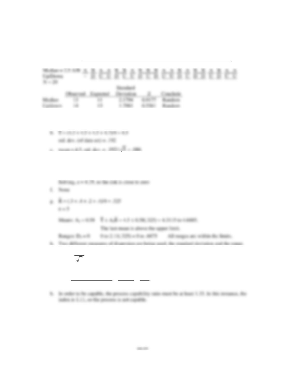
20.
a.
1
2
3
4
4.3
4.5
4.5
4.7
d. 4.5 ± 3(.086) = 4.5 ± .258 = 4.242 to 4.758
The risk is 2(.0013) = .0026
e. 4.5 + z(.086) = 4.86
i.
16.4241.4.4
5
18.0
34.4 ==
to 4.64. The last value is above the upper limit.
21. Solution
a.
11.1
018.
02.
)003(.6
02.
widthprocess
ion widthspecificat
Cp====
Chapter 10 – Quality Control
10–16
22.
Process
Standard Deviation (in.)
Job Specification (in.)
Cp
Capable ?
001
0.02
0.05
0.833
No
003
0.10
0.18
0.600
No
004
0.05
0.15
1.000
No
005
0.01
0.04
1.333
Yes
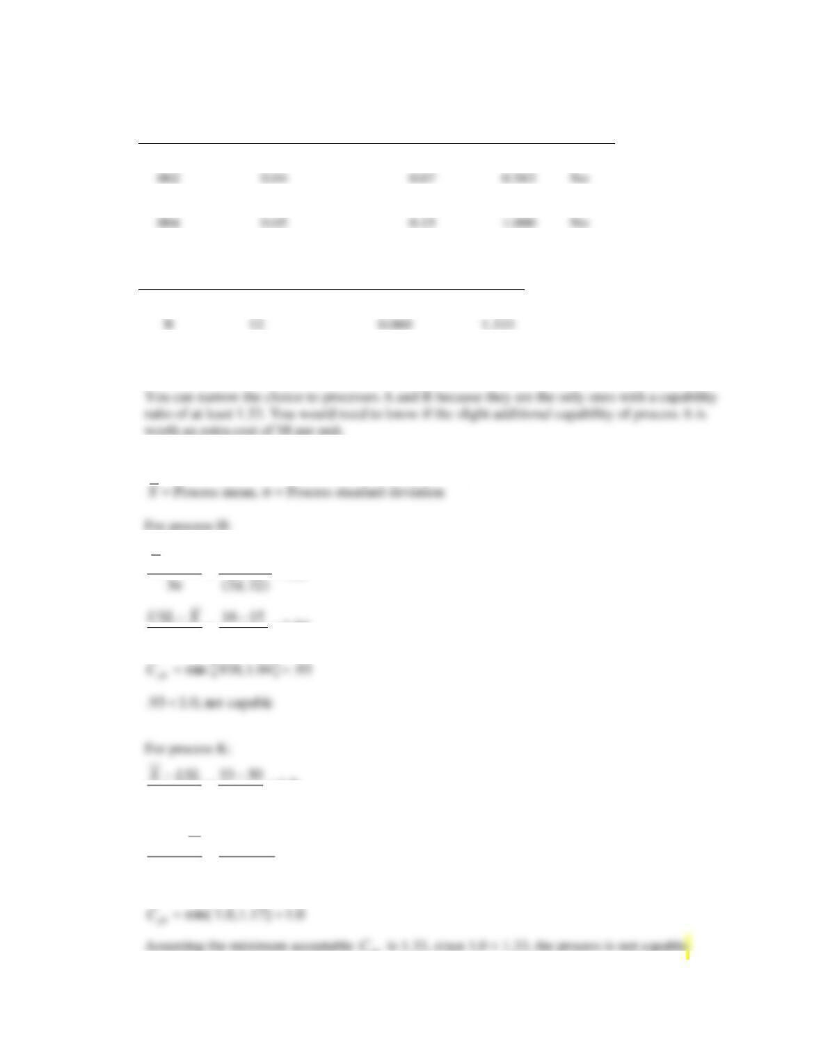
23.
Process
Cost per unit ($)
Standard Deviation (mm.)
Cp
A
20
0.059
1.355
C
11
0.063
1.27
D
10
0.061
1.311
24. Let USL = Upper Specification Limit, LSL = Lower Specification Limit,
04.1
)32)(.3(
3
93.
1.1415
=
=
=
−
=
−
LSLX
17.1
)1)(3(
335.36
3
0.1
)1)(3(
3
=
−
=
−
=
=
XUSL
pk
C
Chapter 10 – Quality Control
10–17
For process T:
33.1
)4.0)(3(
5.181.20
3
=
−
=
−
XUSL
25. Let USL = Upper Specification Limit, LSL = Lower Specification Limit,
X
= Process mean, = Process standard deviation.
For the first repair firm:
0.2
)0.4)(3(
5074
3
=
−
=
−
LSLX
Since 1.333 = 1.333, the firm 1 is capable.
18.1
)1.5)(3(
3
44.1
=
=
=
=
pk
C
Chapter 10 – Quality Control
10–18
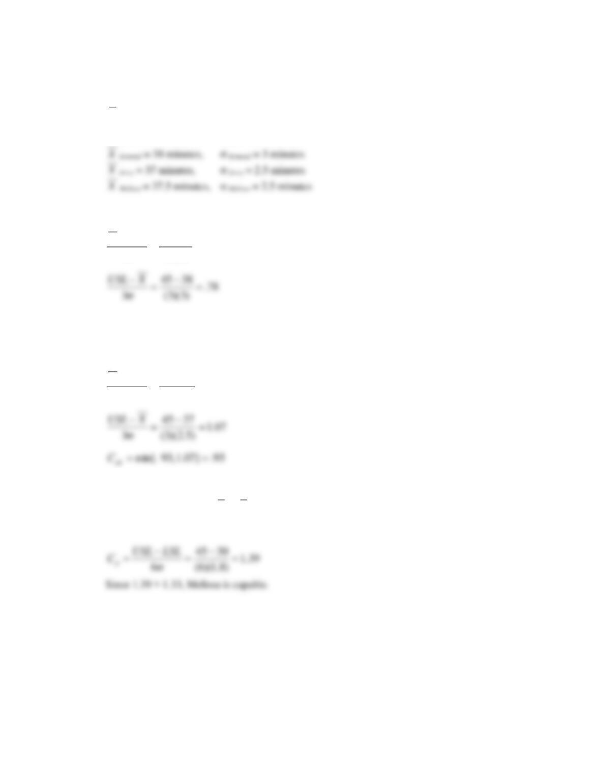
26. Let USL = Upper Specification Limit, LSL = Lower Specification Limit,
X
= Process mean, = Process standard deviation.
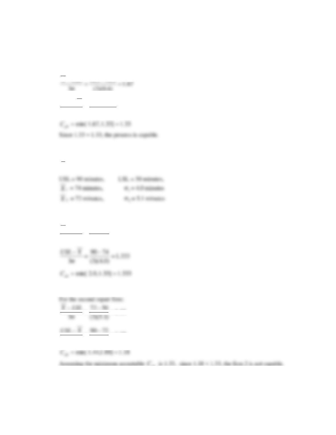
USL = 30 minutes, LSL = 45 minutes,
For Armand:
78.}78.,89min{.
89.
)3)(3(
3038
3
==
=
−
=
−
C
LSLX
pk
Since .78 < 1.33, Armand is not capable.
For Jerry:
93.
)5.2)(3(
3037
3
=
−
=
−
LSLX
Since .93 < 1.33, Jerry is not capable.
For Melissa, since
5.7=−=− LSLXXUSL
, the process is centered, therefore we will use Cp
to measure process capability.
Chapter 10 – Quality Control
10–19
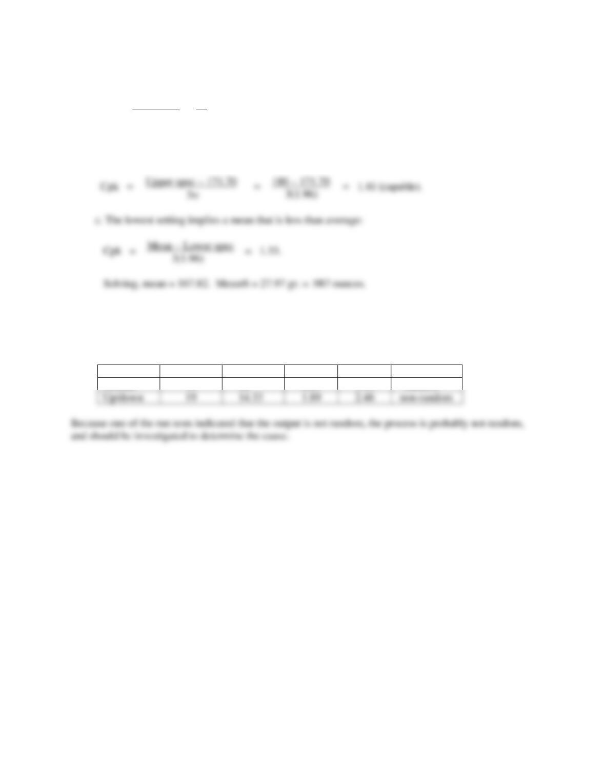
27.
a. Cp = spec width = 20 = 1.33. Solving, = 2.506.
6 6
b. Box variance = 3.84; box = 1.96. Average box weight = 6(1.01) = 6.06 ounces. Students can
deduce that 1 ounce = 28.33 grams, making the box weight in grams: 6.06(28.33) = 171.70 gr.
28. Note that all points are within the control limits, so the process is apparently in control.
Run tests:
Test
Observed
Expected
Std. dev.
Z
Conclusion
Median
15
12
2.29
1.31
random
Solving, mean = 167.82. Mean/6 = 27.97 gr. = .987 ounces.
Chapter 10 – Quality Control
10–20
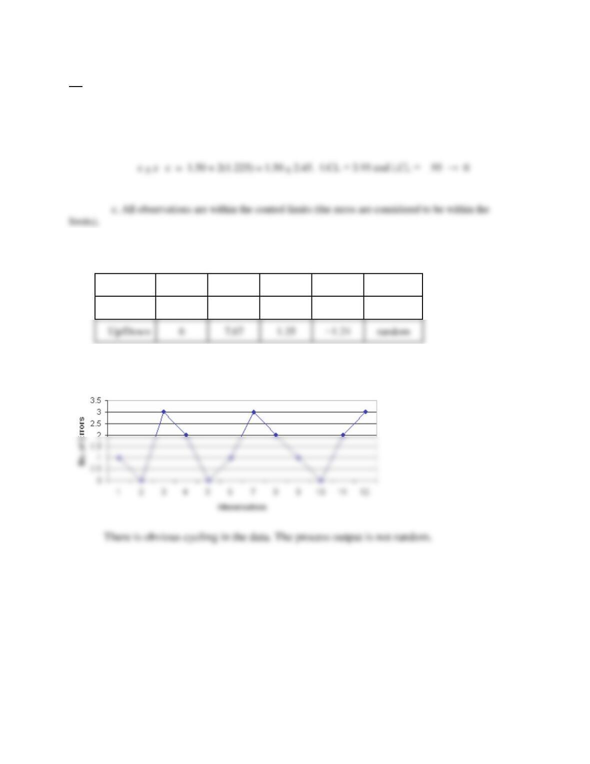
29.
Step 1: a. A c chart is appropriate.
b. The mean of the data is c = 18/12 = 1.50. Control limits are
Step 2: Conduct run tests:
Test
r
expected
Std. dev.
z-score
Conclusion
Median
6
7.00
1.66
−0.60
random
Up/Down
6
7.67
1.35
random
Step 3: Plot the data:

Chapter 10 – Quality Control
10–21
Case: Toys Inc.
A consultant must consider the long-term implications of decisions suggested by management.
2. The trade-in and repair program, while appeasing customers in the short run, may be too costly
and will not be correcting the root cause of the problem.
3. Since the company thrives on its reputation of high quality products, it needs to continue to
4. If implemented well, this strategy will enable the company to become more competitive in the
long run.
Case: Tiger Tools
1. For the first data set
R
= .873. From Table 10–2, for n = 20, A2 = .18. Using the hint, the
estimated standard deviation is .234:
Solving, we obtain
( )
234.20
3
)873)(.18(. ==
2. The process seems to be cycling, as indicated by the control chart for the smaller sample size.
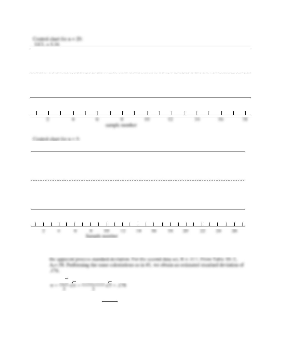
Chapter 10 – Quality Control
10–22
sample number
2 4 6 8 10 12 14 16 18
3. If the cycling can be removed. The true process standard deviation is probably much smaller than
The process capability is
.35.1
)178(.6
44.1 =
Because this is more than 1.33, the process is capable.
LCL = 4.86
•
•
•
•
•
•
•
•
•
•
•
•
•
•
•
•
•
•
UCL = 5.24
LCL = 4.76
Sample number
2 4 6 8 10 12 14 16 18 20 22 24 26
•
•
•
•
•
•
•
•
•
•
•
•
•
•
•
•
•
•
•
•
•
•
•
•
•
•
•
UCL = 5.16

Chapter 10 – Quality Control
10–23
4. Small samples tend to be less reliable than large samples (the standard deviation of the sampling