Distribution and Network ModelsProcesses
10 – 17
Min
8
x
14
6
x
15
+
+
3
x
24
8
x
25
+
9
x
34
3
x
35
+
44
x
46
+
34
x
47
34
x
48
32
x
49
+
+
+
+
57
x
56
+
35
x
57
+
28
x
58
+
24
x
59
+
s.t.
x
14
x
15
+
=
=
=
0
+
15
–
35
x
56
x
57
58
59
25
=
3
3
4
2
3
x
46
x
47
x
48
x
49
x
56
x
57
x
58
x
59
x
ij
0 for all
i, j
+
+
+
+
Optimal Solution Units Shipped Cost
Muncie to Cincinnati 1 6
Cincinnati to Concord 3 84
Two rail cars must be held at Muncie until a buyer is found.
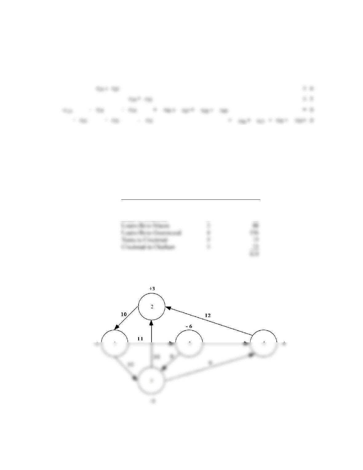
15.
The positive numbers by nodes indicate the amount of supply at that node. The negative numbers by
nodes indicate the amount of demand at the node.
Chapter 10
16. a.
Min
s.t.
20x12 +25x15
30x42
x12
–
x15
x31 –
= 8
+
+
30x25
25x53
+
+
45x27
15x54
+
+
20x31
28x56
+
+
35x36
12x67 +27x74
+
10 – 19
b. x12 = 0 x53 = 5
x15 = 0 x54 = 0
x25 = 8 x56 = 5
Total cost of redistributing cars = $917
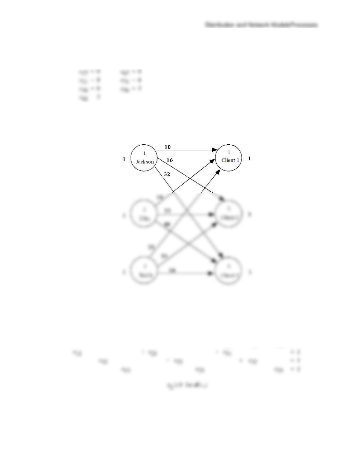
17. a.
b.
Min
10x11
+
16x12
+
32x13
+
14x21
+
22x22
+
40x23
+
22x31
+
24x32
+
34x33
s.t.
x11
+
x12
+
x13
1
x21
+
x22
+
x23
1
x31
+
x32
+
x33
1
x11
x21
+
x31
=
1
x12
+
x22
+
x32
=
1
+
+
x33
=
1
Solution x12 = 1, x21 = 1, x33 = 1 Total completion time = 64
Chapter 10
10 – 20
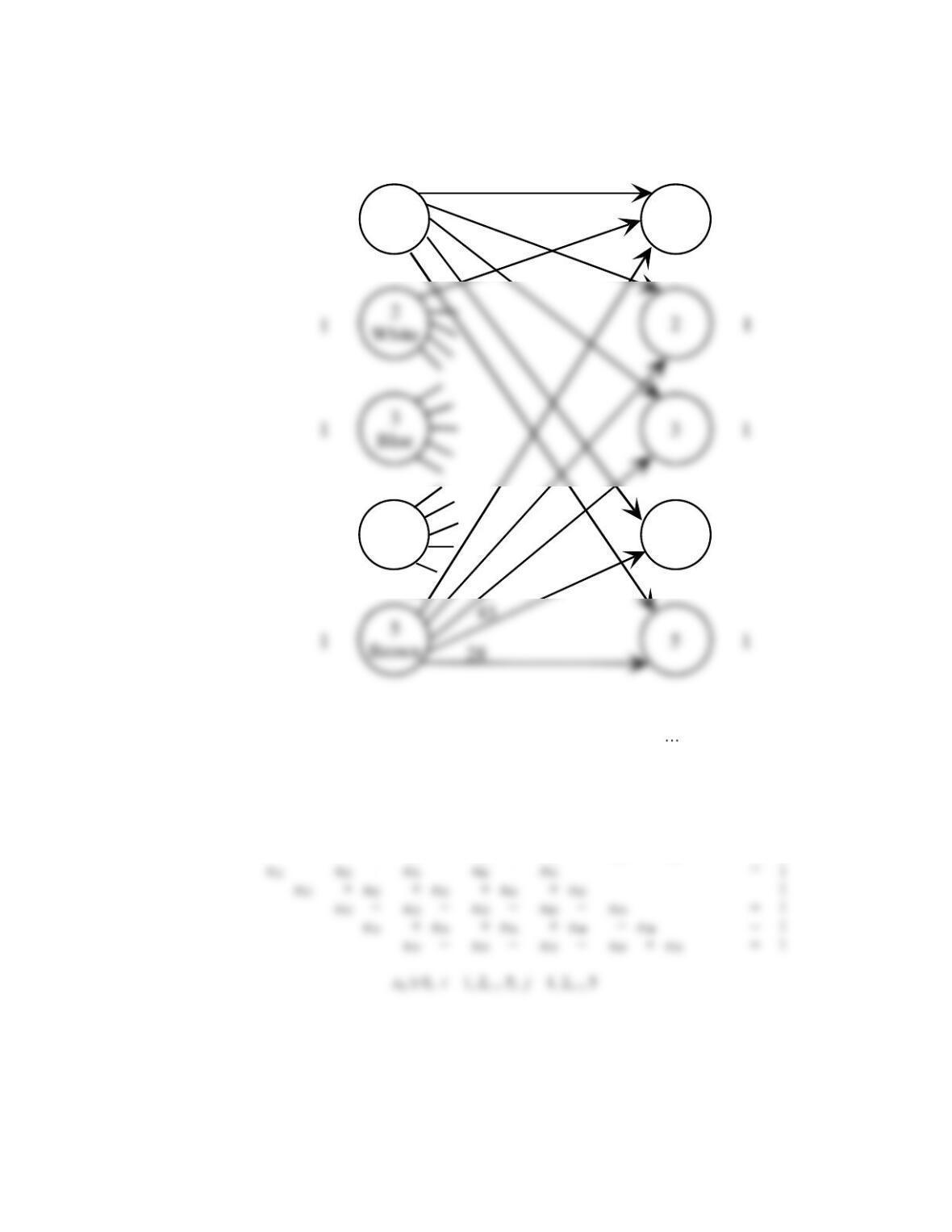
18. a.
b.
Min
30x11
+
44x12
+
38x13
+
47x14
+
31x15
+
25x21
+
+
28x55
s.t.
x11
+
x12
+
x13
+
x14
+
x15
1
x21
+
x22
+
x23
+
x24
+
x25
1
x31
+
x32
+
x33
+
x34
+
x35
1
x41
+
x42
+
x43
+
x44
+
x45
1
x51
+
x52
+
x53
+
x54
+
x55
1
x11
+
x21
+
x31
+
x41
+
x51
=
1
x12
+
x22
+
x32
+
x42
+
x52
=
1
x13
+
x23
+
x33
+
x43
+
x53
=
1
x14
+
x24
+
x34
+
x44
+
x54
=
1
x15
+
x25
+
x35
+
x45
+
x55
=
1
4
Green
1
Red
1
4
44
34
25
26
30
44
38
47
Crews Jobs
1
1
11
Distribution and Network ModelsProcesses
10 – 21
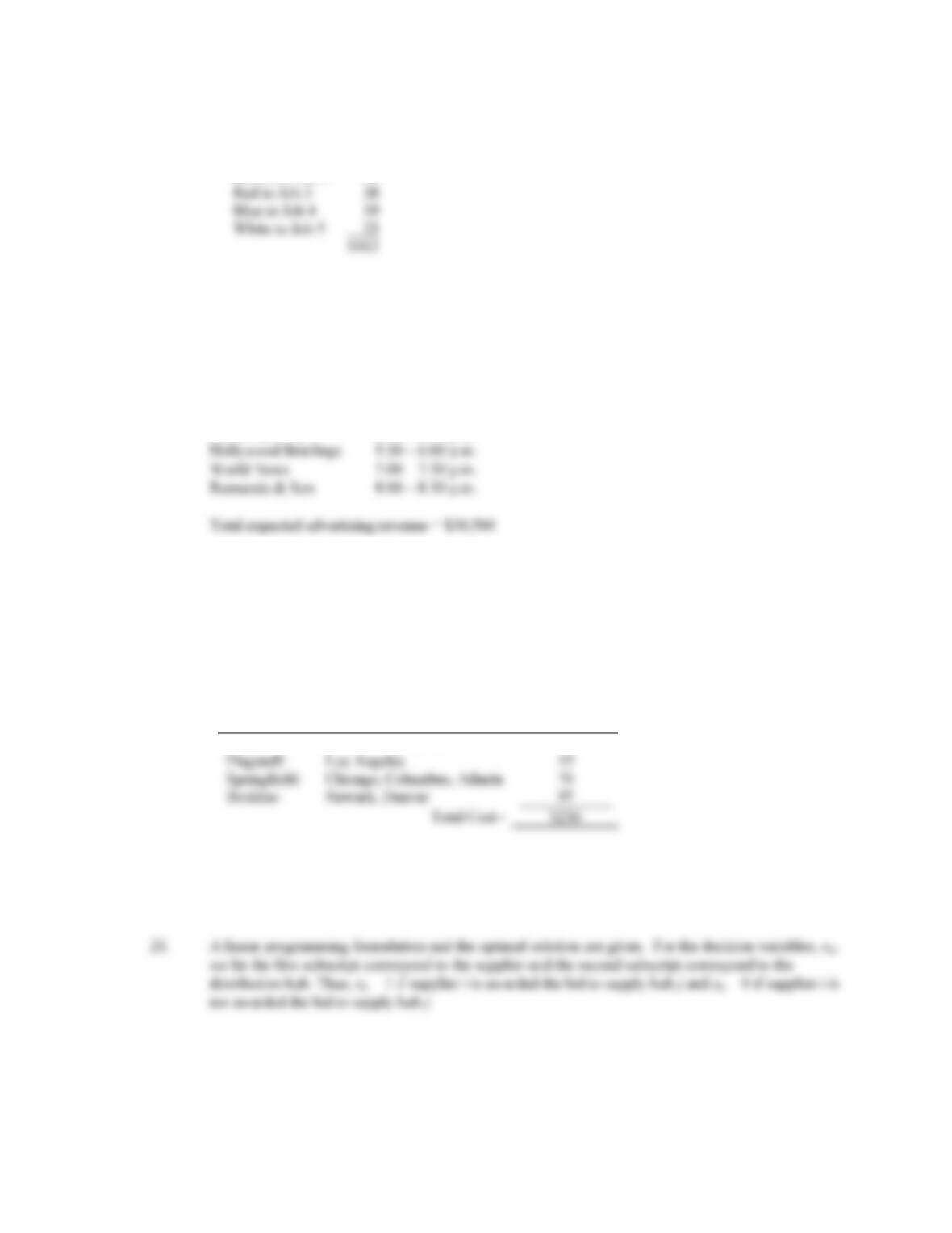
Optimal Solution:
Green to Job 1
$26
Brown to Job 2
Red to Job 3
Blue to Job 4
White to Job 5
Since the data is in hundreds of dollars, the total installation cost for the 5 contracts is $16,200.
19. This can be formulated as a linear program with a maximization objective function. There are 24
variables, one for each program/time slot combination. There are 10 constraints, 6 for the potential
programs and 4 for the time slots.
Optimal Solution:
NASCAR Live 5:00 – 5:30 p.m.
20. a. This is the variation of the assignment problem in which multiple assignments are possible. Each
distribution center may be assigned up to 3 customer zones.
The linear programming model of this problem has 40 variables (one for each combination of
distribution center and customer zone). It has 13 constraints. There are 5 supply ( 3) constraints
and 8 demand (= 1) constraints.
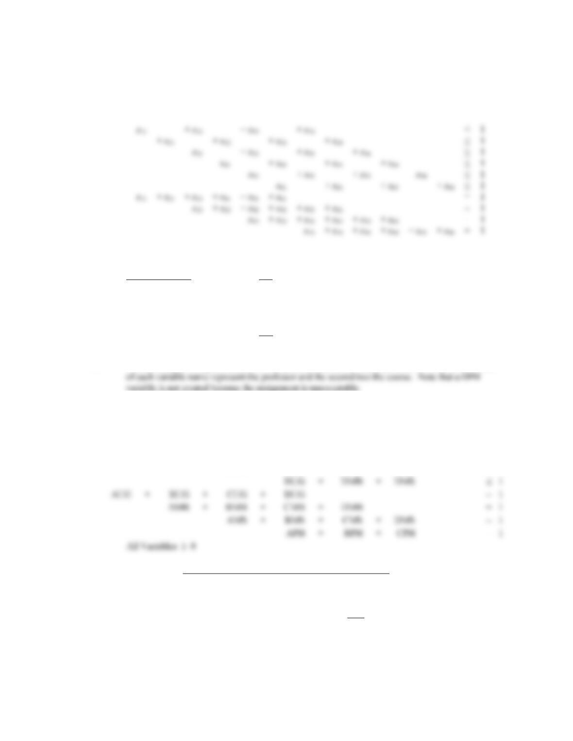
The optimal solution is given below.
Assignments
Cost ($1000s)
Plano:
Kansas City, Dallas
34
Flagstaff:
Los Angeles
15
Springfield:
Chicago, Columbus, Atlanta
70
b. The Nashville distribution center is not used.
c. All the distribution centers are used. Columbus is switched from Springfield to Nashville. Total
cost increases by $11,000 to $227,000.
Chapter 10
10 – 22
Min 190x11 +175x12 + 125x13 + 230x14 + 150x21 + 235x22 + 155x23 + 220x24 + 210x31 + 225x32
+ 135x33 +260x34 + 170x41 + 185x42 + 190x43 + 280x44 + 220x51 + 190x52 + 140x53
+ 240x54 + 270x61 + 200x62 + 130x63 + 260x64
s.t.
xij 0 for all i, j
Optimal Solution Bid
Martin – Hub 2 175
Schmidt Materials – Hub 4 220
D&J Burns – Hub 1 170
Lawler Depot – Hub 3 130
695
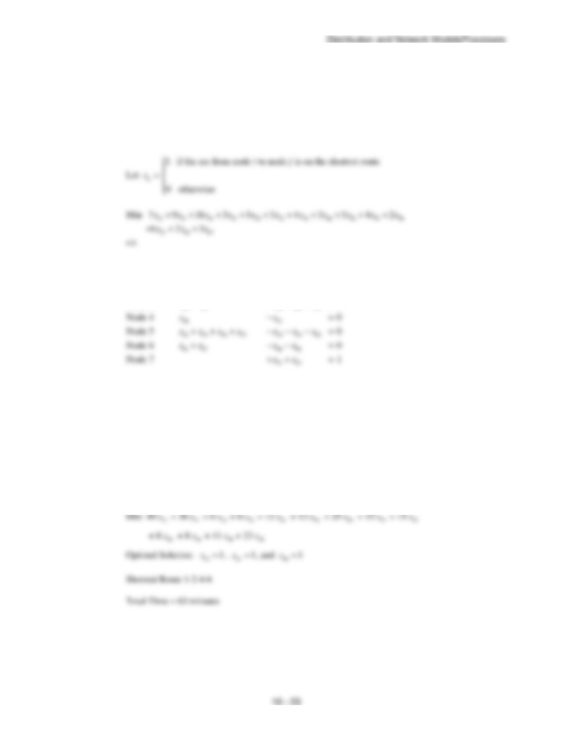
22. A linear programming formulation of this problem can be developed as follows. Let the first letter
Max
2.8AUG
+
2.2AMB
+
3.3AMS
+
3.0APH
+
3.2BUG
+
· · ·
+
2.5DMS
s.t.
AUG
+
AMB
+
AMS
+
APH
1
BUG
+
BMB
+
BMS
+
BPH
1
CUG
+
CMB
+
CMS
+
CPH
1
DUG
+
DMB
+
DMS
1
AUG
+
BUG
+
CUG
+
DUG
=
1
AMB
+
BMB
+
CMB
+
DMB
=
1
AMS
+
BMS
+
CMS
+
DMS
=
1
APH
+
BPH
+
CPH
=
1
Optimal Solution:
Rating
A to MS course
3.3
B to Ph.D. course
3.6
C to MBA course
3.2
D to Undergraduate course
3.2
Max Total Rating
13.3
23. Origin – Node 1
Transshipment Nodes 2 to 5
Destination – Node 7
The linear program will have 14 variables for the arcs and 7 constraints for the nodes.
Flow Out Flow In
Node 1
12 13 14
x x x++
= 1
Node 2
23 25
xx
+
12 32 52
x x x
− − −
= 0
Node 3
xx
+
x x x
− − −
= 0
ij
x
> 0 for all i and j
Optimal Solution:
12 1x=
,
25 1x=
,
56 1x=
, and
67 1x=
Shortest Route 1-2-5-6-7
Length = 17
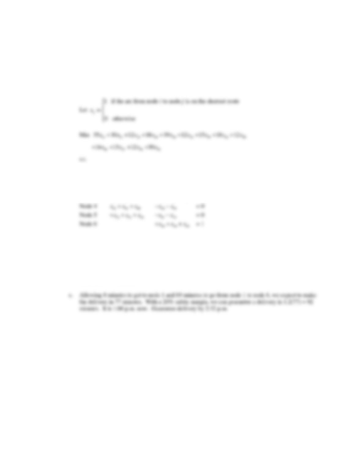
24. The linear program has 13 variables for the arcs and 6 constraints for the nodes. Use same six
constraints for the Gorman shortest route problem as shown in the text. The objective function
changes to travel time as follows.
Chapter 10
10 – 24
25. a. Origin – Node 1
Transshipment Nodes 2 to 5
Destination – Node 6
The linear program will have 13 variables for the arcs and 6 constraints for the nodes.
Flow Out Flow In
Node 1
12 13
xx
+
= 1
Node 2
23 24 26
x x x
++
12 32 42
x x x
− − −
= 0
Node 3
32 35
xx
+
13 23 53
x x x
− − −
= 0
ij
x
> 0 for all I and j
b. Optimal Solution:
12 1x=
,
24 1x=
, and
46 1x=
Shortest Route 1-2-4-6
Total time = 69 minutes
10 – 25
26. Origin – Node 1
Transshipment Nodes 2 to 5 and node 7
Destination – Node 6
The linear program will have 18 variables for the arcs and 7 constraints for the nodes.
s.t.
Flow Out Flow In
Node 1
12 13 14
x x x++
= 1
Node 2
23 25
xx
+
12 32 52
x x x
− − −
= 0
Node 3
32 34 35 36
x x x x+ + +
13 23 43 53
x x x x− − − −
= 0
52 53 56 57
x x x x+ + +
ij
x
> 0 for all i and j
Optimal Solution:
14 1x=
,
47 1x=
, and
76 1x=
Shortest Route 1-4-7-6
Total Distance = 40 miles
Chapter 10
10 – 26
27. Origin – Node 1
Transshipment Nodes 2 to 9
Destination – Node 10 (Identified by the subscript 0)
The linear program will have 29 variables for the arcs and 10 constraints for the nodes.
Flow Out Flow In
Node 1
12 13 14 15
x x x x
+ + +
= 1
Node 2
23 27
xx+
12 32 72
x x x
− − −
= 0
Node 3
32 36
xx
+
13 23 43 63
x x x x− − − −
= 0
Node 4
43 45 46
x x x
++
14 54 64
x x x
− − −
= 0
Node 5
54 59
xx
+
15 45 95
x x x
− − −
= 0
ij
x
> 0 for all i and j
Optimal Solution:
15 1x=
,
54 1x=
,
46 1x=
,
67 1x=
, and
70 1x=
10 – 27
28. Origin – Node 0
Transshipment Nodes 1 to 3
Destination – Node 4
The linear program will have 10 variables for the arcs and 5 constraints for the nodes.
s.t.
Flow Out Flow In
Node 0
01 02 03 04
x x x x+ + +
= 1
Node 1
12 13 14
x x x++
01
x−
= 0
Node 2
23 24
xx
+
02 12
xx−−
= 0
Node 3
34
x
03 13 23
x x x
− − −
= 0
Node 4
04 14 24 34
x x x x− − − −
= 1
ij
x
> 0 for all i and j
29. The capacitated transshipment problem to solve is given:
Max x61
s.t.
x12 + x13 + x14 – x61 = 0
x24 + x25 – x12 – x42 = 0
x34 + x36 – x13 – x43 = 0
x42 + x43 + x45 + x46 – x14 – x24 – x34 – x54 = 0
x54 + x56 – x25 – x45 = 0
x61 – x36 + x46 – x56 = 0
Chapter 10
10 – 28
3
3
2
5
2
2
3
1
1
4
30.
31. The maximum number of messages that may be sent is 10,000.
32. a. 10,000 gallons per hour or 10 hours
b. Flow reduced to 9,000 gallons per hour; 11.1 hours.
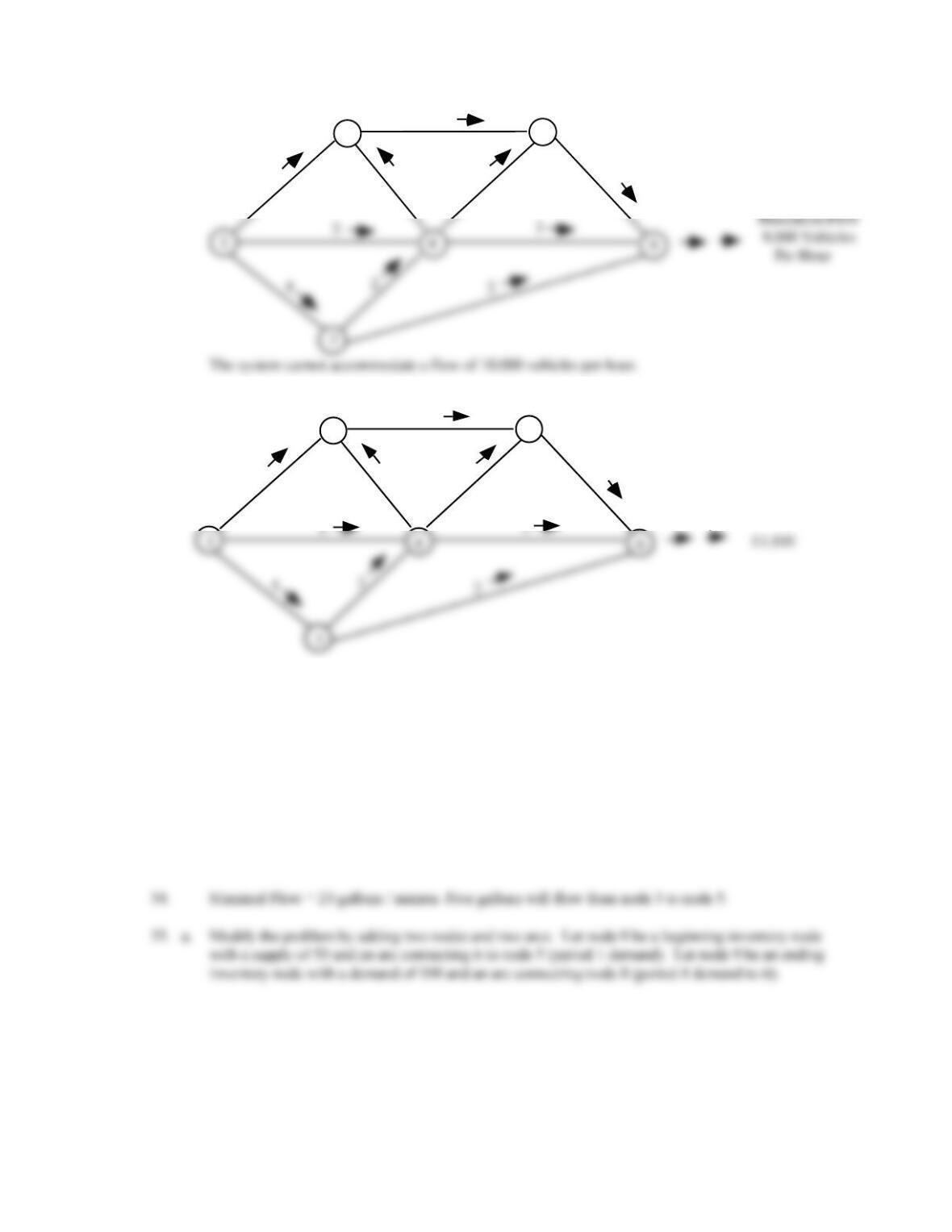
33. Current Max Flow = 6,000 vehicles/hour.
With arc 3-4 at a 3,000 unit/hour flow capacity, total system flow is increased to 8,000 vehicles/hour.
Increasing arc 3-4 to 2,000 units/hour will also increase system to 8,000 vehicles/hour. Thus a 2,000
unit/hour capacity is recommended for this arc.
5
2
3
4
21
6
10 – 29
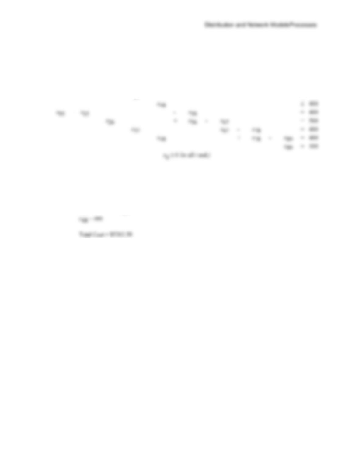
b.
Min
+
2x15
+
5x26
+
3x37
+
3x48
+
0.25x56
+
0.25x67
+
0.25x78
+
0.25x89
s.t.
x05
=
50
x15
600
x26
300
400
x05
+
x15
–
=
400
x26
+
–
=
500
x37
+
–
=
400
+
–
=
400
=
100
x37
500
Optimal Solution:
x05 = 50 x56 = 250
x15 = 600 x67 = 0
x26 = 250 x78 = 100
x37 = 500 x89 = 100
Chapter 10
10 – 30
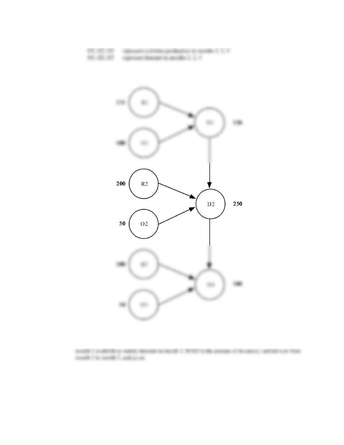
36. a. Let R1, R2, R3 represent regular time production in months 1, 2, 3
Using these 9 nodes, a network model is shown.
b. Use the following notation to define the variables: first two letters designates the “from node” and
the second two letters designates the “to node” of the arc. For instance, R1D1 is amount of regular
time production available to satisfy demand in month 1, O1D1 is amount of overtime production in
10 – 31
MIN 50R1D1 + 80O1D1 + 20D1D2 + 50R2D2 + 80O2D2 + 20D2D3 + 60R3D3 + 100O3D3
S.T.
1) R1D1 275
2) O1D1 100
3) R2D2 200
4) O2D2 50
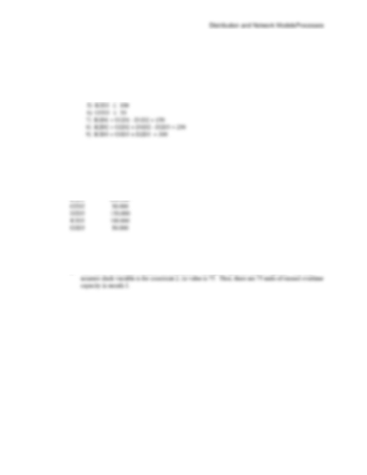
c. Optimal Solution:
Variable Value
————– —————
R1D1 275.000
O1D1 25.000
D1D2 150.000
Value = $46,750
Note: Slack variable for constraint 2 = 75.
d. The values of the slack variables for constraints 1 through 6 represent unused capacity. The only
Chapter 10
10 – 32