Markov Processes
17 – 1
Chapter 10
Distribution and Network Models
Learning Objectives
1. Understand the usefulness of using optimization for supply chain problems.
2. Be able to identify the special features of the transportation problem.
6. Be able to identify the special features of the assignment problem.
7. Become familiar with the types of problems that can be solved by applying an assignment model.
8. Be able to develop network and linear programming models of the assignment problem.
9. Be familiar with the special features of the transshipment problem.
10. Become familiar with the types of problems that can be solved by applying a transshipment model.
14. Know the basic characteristics of the maximal flow problem.
15. Be able to develop a linear programming model and solve the maximal flow problem.
16. Know how to structure and solve a production and inventory problem as a transshipment problem.
17. Understand the following terms:
network flow problem
capacitated transshipment problem
transportation problem
shortest route
origin
maximal flow
destination
source node
capacitated transportation problem
sink node
assignment problem
arc flow capacities
Chapter 10
10 – 2
Solutions:
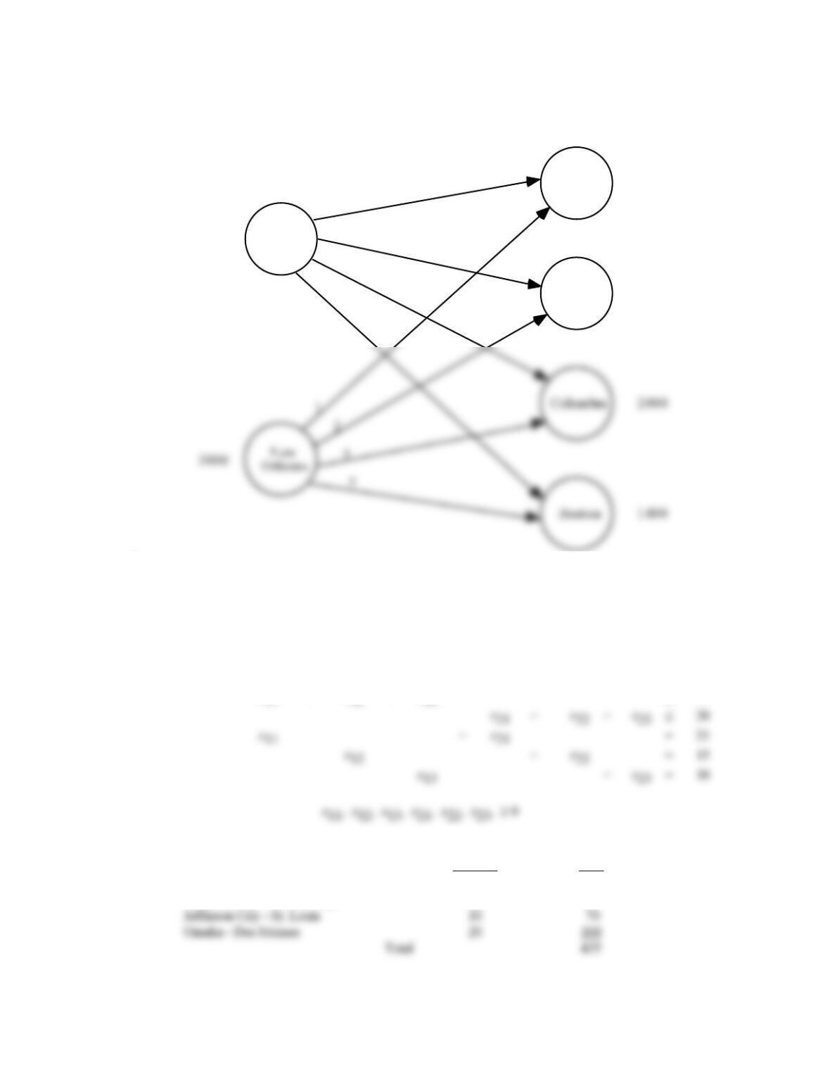
1. The network model is shown.
2. a.
Let
x11
:
Amount shipped from Jefferson City to Des Moines
x12
:
Amount shipped from Jefferson City to Kansas City
•
•
•
Min
14x11
+
9x12
+
7x13
+
8x21
+
10x22
+
5x23
s.t.
20
x11
+
=
x12
15
x13
+
=
x11
+
x12
+
x13
30
b. Optimal Solution:
Amount
Cost
Jefferson City – Des Moines
5
70
Jefferson City – Kansas City
15
135
Jefferson City – St. Louis
10
70
P hila.
Dallas
Atlan t a
5000
2
6
6
2
3200
1400
10 – 3
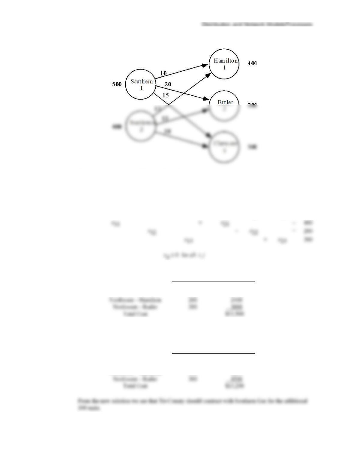
3. a.
b. Let xij = amount shipped from supply node i to demand node j.
Min
10x11
+
20x12
+
15x13
+
12x21
+
15x22
+
18x23
s.t.
x11
+
x12
+
x13
500
x21
+
x22
+
x23
400
+
x21
=
x12
+
x22
=
200
+
=
300
c. Optimal Solution
Amount
Cost
Southern – Hamilton
200
$ 2000
Southern – Clermont
300
4500
200
2400
200
3000
$11,900
d. To answer this question the simplest approach is to increase the Butler County demand to 300 and to
increase the supply by 100 at both Southern Gas and Northwest Gas. The new optimal solution is:
Amount
Cost
Southern – Hamilton
300
$ 3000
Southern – Clermont
300
4500
100
1200
300
4500
$13,200
Chapter 10
10 – 4
4.
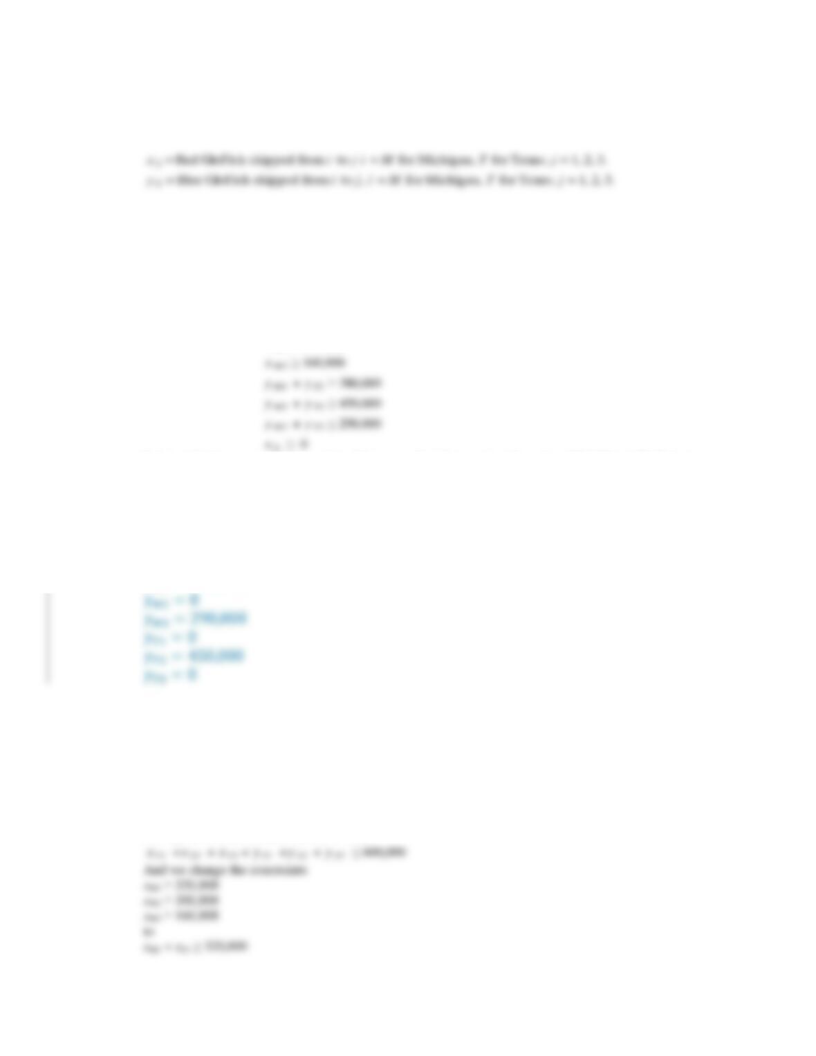
a. The optimization model can be written as
Minimize xM1 + 2.50x M2 + 0.50x M3 + y M1 + 2.50y M2 + 0.50y M3 + 2.00y T1 + 1.50y T2 + 2.80y T3
subject to
xM1 + x M2 + x M3 ≤ 1,000,000
yM1 + y M2 + y M3 ≤ 1,000,000
yT1 +y T2 + y T3 ≤ 600,000
xM1 ≥ 320,000
xM2 ≥ 300,000
xM3 ≥ 160,000
yM1 + y T1 ≥ 380,000
yM3 + y T3 ≥ 290,000
xij ≥ 0
Solving this linear program using Excel Solver we find that we should produce 780,000 red GloFish in
Michigan, 670,000 blue GloFish in Michigan, and 450,000 blue GloFish in Texas.
Using the notation in the model, the number of GloFish shipped from each farm to each retailer can be
expressed as:
𝑥𝑀1 =320,000
𝑥𝑀2 =300,000
𝑥𝑀3 =160,000
𝑦𝑀1 =380,000
b. From Excel Solver, the minimum transportation cost is $2.35 million.
c. We have to add variables xT1, xT2 and xT3 for Red GloFish shipped between Texas and Retailers 1, 2
and 3. The revised objective function is
Minimize xM1 + 2.50x M2 + 0.50x M3 + y M1 + 2.50y M2 + 0.50y M3 + 2.00y T1 + 1.50y T2 + 2.80y T3
+ x T1 + 2.50x T2 + 0.50x T3
We replace the third constraint above with
10 – 5
xM2 + xT2 ≥ 300,000
xM3 + xT3 ≥ 160,000
Using this new objective function and constraint the optimal solution is $2.2 million, so the savings are
$150,000.
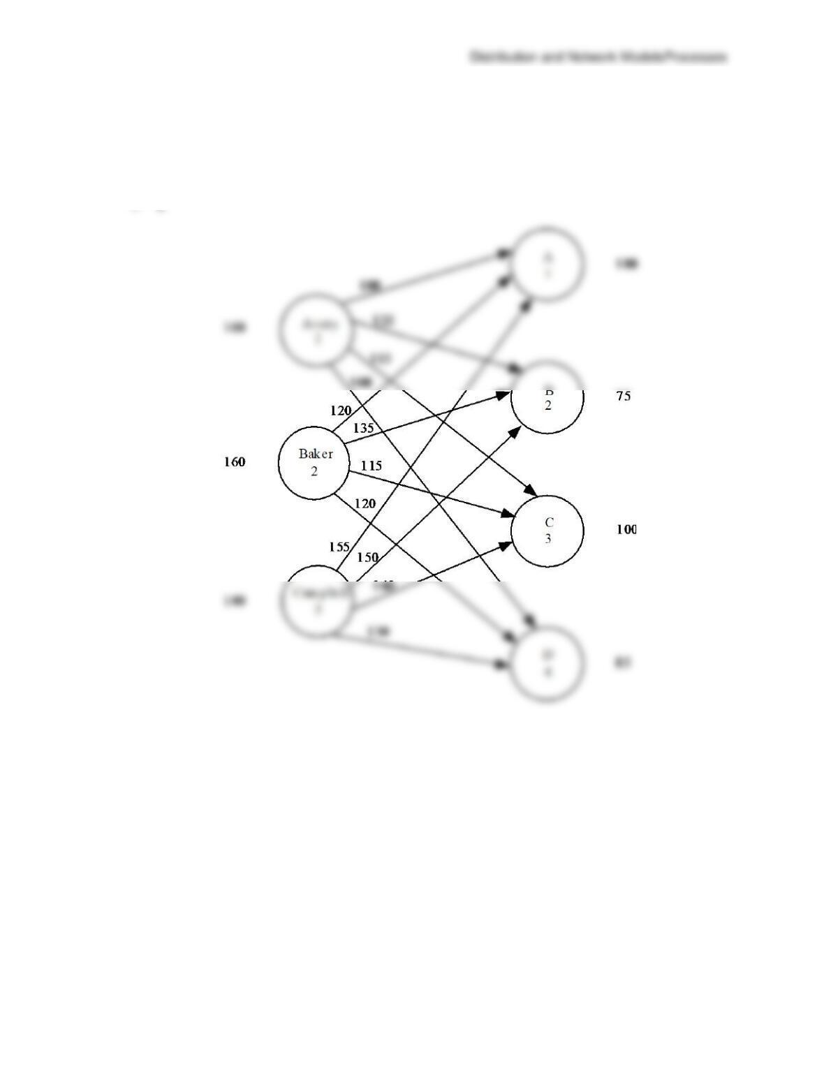
b. Let xij = number of hours from consultant i assigned to client j.
Chapter 10
10 – 6
Max
100x11
+
125x12
+
115x13
+
100x14
+
120x21
+
135x22
+
115x23
+
120x24
+
155x31
+
150x32
+
140x33
+
130x34
s.t.
x11
+
x12
+
x13
+
x14
160
x21
+
x22
+
x23
+
x24
160
x31
+
x32
+
x33
+
x34
140
x11
+
x21
+
x31
=
180
x12
+
x22
+
x32
=
x13
+
x23
+
x33
=
100
x14
+
x24
+
x34
=
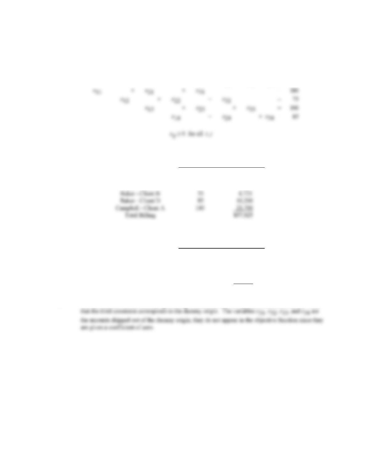
Optimal Solution
Hours
Assigned
Billing
Avery – Client B
40
$ 5,000
Avery – Client C
100
11,500
Baker – Client A
40
4,800
Baker – Client B
35
4,725
Baker – Client D
85
10,200
Campbell – Client A
140
21,700
Total Billing
$57,925
c. New Optimal Solution
Hours
Assigned
Billing
Avery – Client A
40
$ 4,000
Avery – Client C
100
11,500
Baker – Client B
75
10,125
Baker – Client D
85
10,200
Campbell – Client A
140
21,700
Total Billing
$57,525
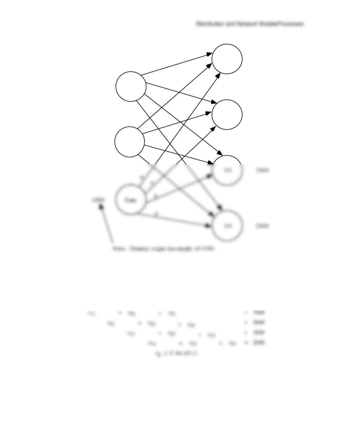
6. The network model, the linear programming formulation, and the optimal solution are shown. Note
10 – 7
Max
32
x
11
34
x
12
+
+
32
x
13
40
x
14
+
34
x
21
30
x
22
28
x
23
38
x
24
+
+
+
+
s.t.
x
11
x
12
+
+
x
13
x
21
x
22
+
+
x
23
x
31
x
32
+
+
x
33
5000
3000
4000
5000
=
x
+
x
+
x
x
Dummy
x
14
+
x
24
+
+
x
34
C.S.
D.
D1
D2
40
32
34
32
38
28
30
34
5000
3000
5000
2000
Supply
Dem and
Chapter 10
10 – 8
Optimal Solution Units Cost
Clifton Springs – D2 4000 $136,000
Clifton Springs – D4 1000 40,000
Customer 2 demand has a shortfall of 1000
Customer 3 demand of 3000 is not satisfied.
7.
a. Let xij = MW produced at plant i for city j; i = L for Los Angeles, T for Tulsa, S for Seattle, j = 1, …, 10.
𝑀𝑖𝑛 356.26𝑥𝐿1 +356.25𝑥𝐿2 +178.13𝑥𝐿3 +356.25𝑥𝐿4 +237.50𝑥𝐿5 +415.63𝑥𝐿6
+356.25𝑥𝐿7 +356.25𝑥𝐿8 +178.13𝑥𝐿9 +356.25𝑥𝐿10 +593.75𝑥𝑇1
subject to
𝑥𝐿1 + 𝑥𝑇1 + 𝑥𝑆1 ≥950.00
𝑥𝐿2 + 𝑥𝑇2 + 𝑥𝑆2 ≥831.25
𝑥𝐿3 + 𝑥𝑇3 + 𝑥𝑠3 ≥2375.00
𝑥𝐿4 + 𝑥𝑇4 + 𝑥𝑆4 ≥593.75
By solving this linear program in Excel Solver, we find the optimal solution is to produce 6412.50 MWs in
Los Angeles, 1543.75 MWs in Tulsa, and 2968.75 MWs in Seattle. The total distribution cost of this
solution is $2,552,382.81.
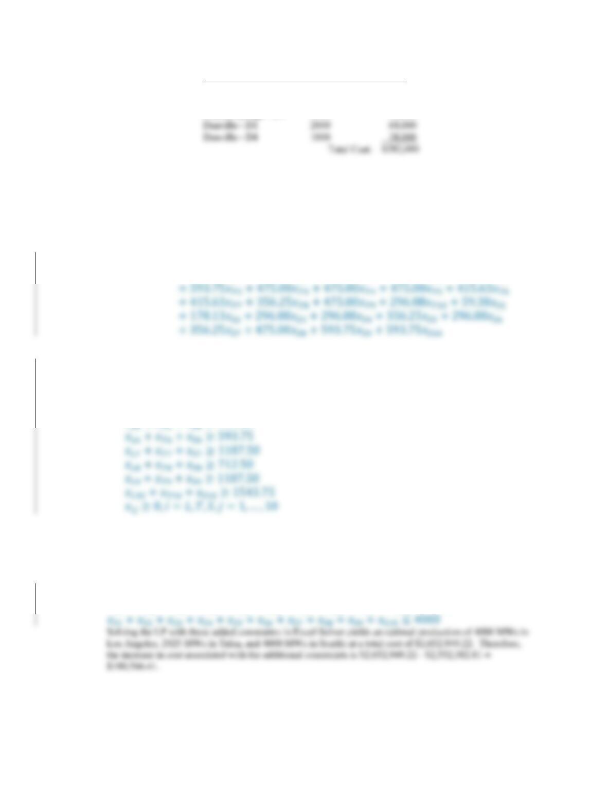
b. We must add the following constraints to the linear program shown above:
𝑥𝐿1 + 𝑥𝐿2 + 𝑥𝐿3 + 𝑥𝐿4 + 𝑥𝐿5 + 𝑥𝐿6 + 𝑥𝐿7 + 𝑥𝐿8 + 𝑥𝐿9 + 𝑥𝐿10 ≤4000
𝑥𝑇1 + 𝑥𝑇2 + 𝑥𝑇3 + 𝑥𝑇4 + 𝑥𝑇5 + 𝑥𝑇6 + 𝑥𝑇7 + 𝑥𝑇8 + 𝑥𝑇9 + 𝑥𝑇10 ≤4000
10 – 9
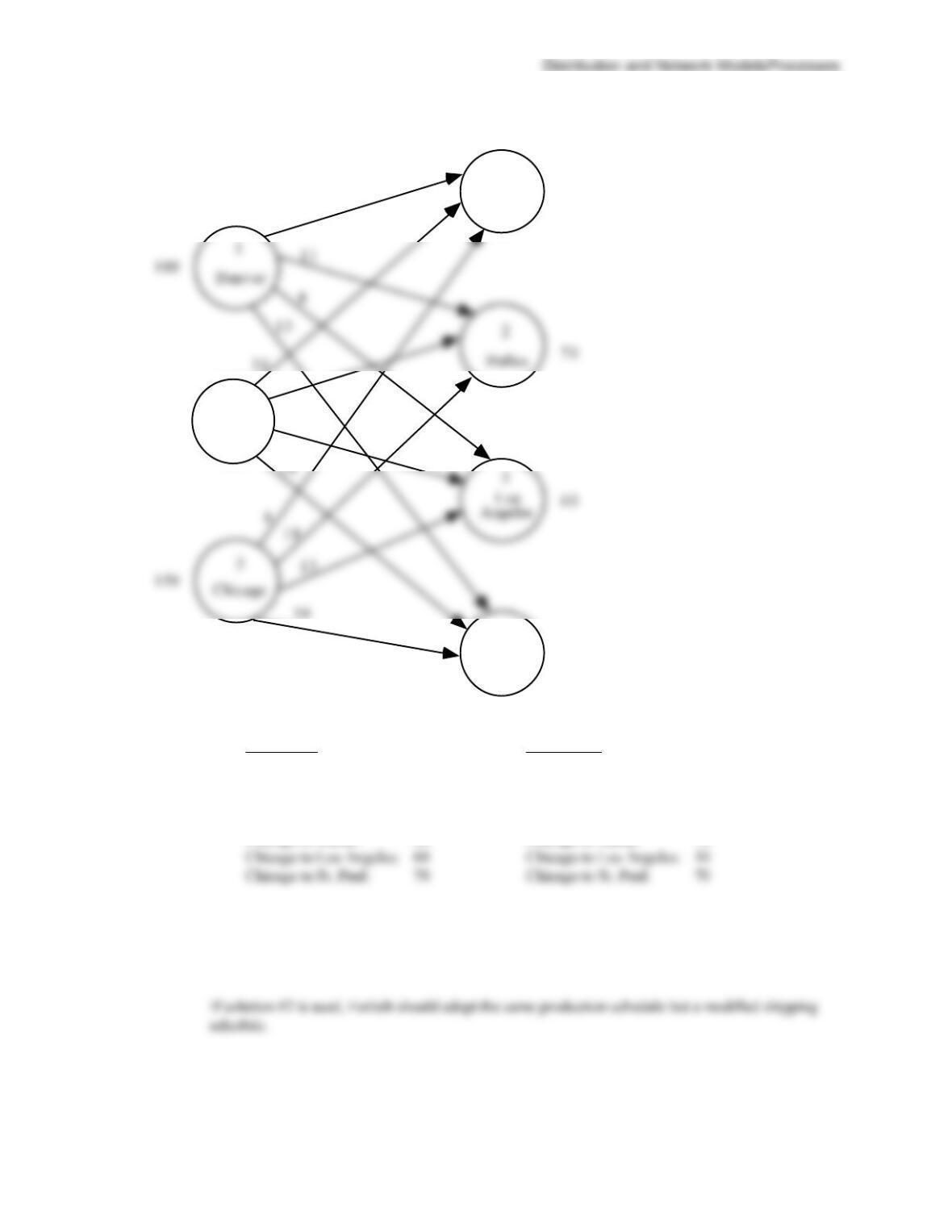
8. a.
b. There are alternative optimal solutions.
Solution #1
Solution # 2
Denver to St. Paul: 10
Denver to St. Paul: 10
Atlanta to Boston: 50
Atlanta to Boston: 50
Atlanta to Dallas: 50
Atlanta to Los Angeles: 50
Chicago to Dallas: 20
Chicago to Dallas: 70
Chicago to Los Angeles: 60
Chicago to Los Angeles: 10
Chicago to St. Paul: 70
Chicago to St. Paul: 70
Total Profit: $4240
If solution #1 is used, Forbelt should produce 10 motors at Denver, 100 motors at Atlanta, and 150
motors at Chicago. There will be idle capacity for 90 motors at Denver.
2
Atlan t a
1
Bost o n
4
St. P aul
7
12
17
100
80
50
Chapter 10
10 – 10
9. The linear programming formulation and optimal solution are shown.
Let
x1A
=
Units of product A on machine 1
x1B
x3C
=
Units of product C on machine 3
Min
x
1A
1.2
x
1B
+
+
0.9
x
1C
1.3
x
2A
+
1.4
x
2B
1.2
x
2C
1.1
x
3A
x
3B
+
+
+
+
s.t.
x
1A
x
1B
+
+
x
1C
x
2A
x
2B
+
+
x
2C
x
3A
x
3B
+
+
x
3C
1500
1500
1000
=
=
x
3B
+
3C
2B
+
+
2C
1B
1C
x
1.2
x
3C
+
Optimal Solution Units Cost
1 – A 300 $ 300
1 – C 1200 1080
2 – A 1200 1560
Note: There is an unused capacity of 300 units on machine 2.
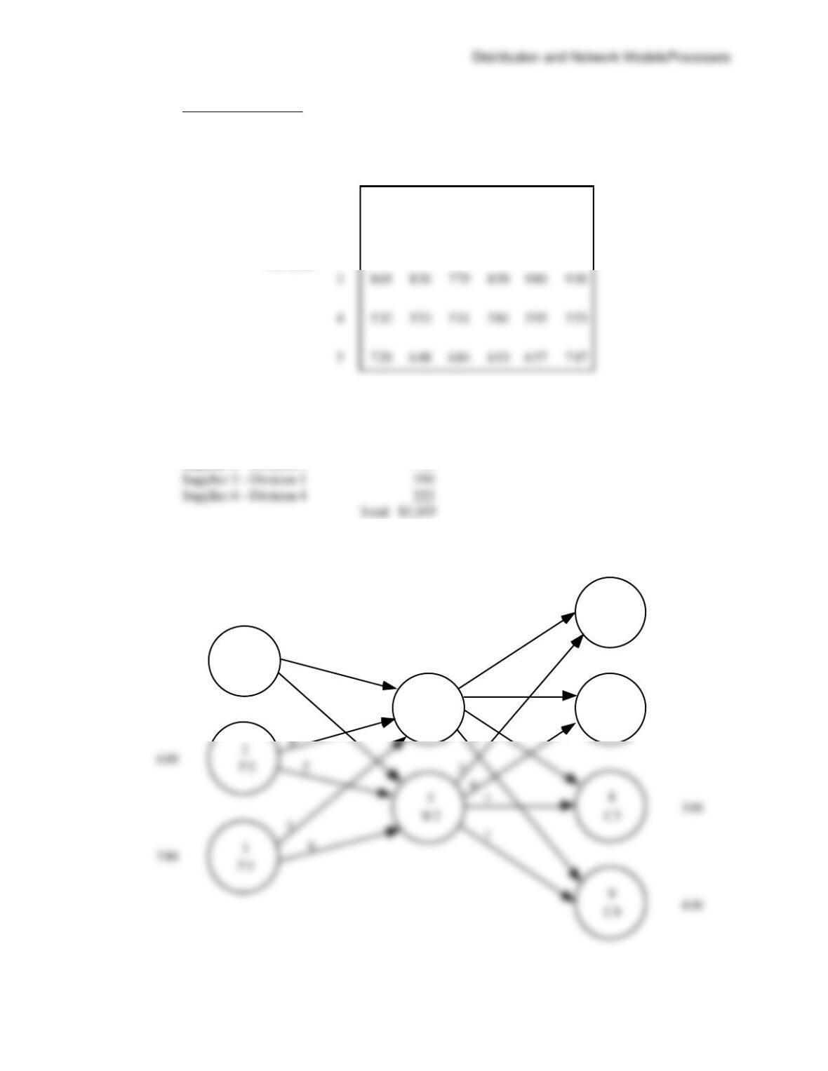
10. a. The total cost is the sum of the purchase cost and the transportation cost. We show the calculation
for Division 1 – Supplier 1 and present the result for the other Division-Supplier combinations.
Division 1 – Supplier 1
10 – 11
Cost Matrix ($1,000s)
b. Optimal Solution:
Supplier 1 – Division 2 $ 603
Supplier 2 – Division 5 648
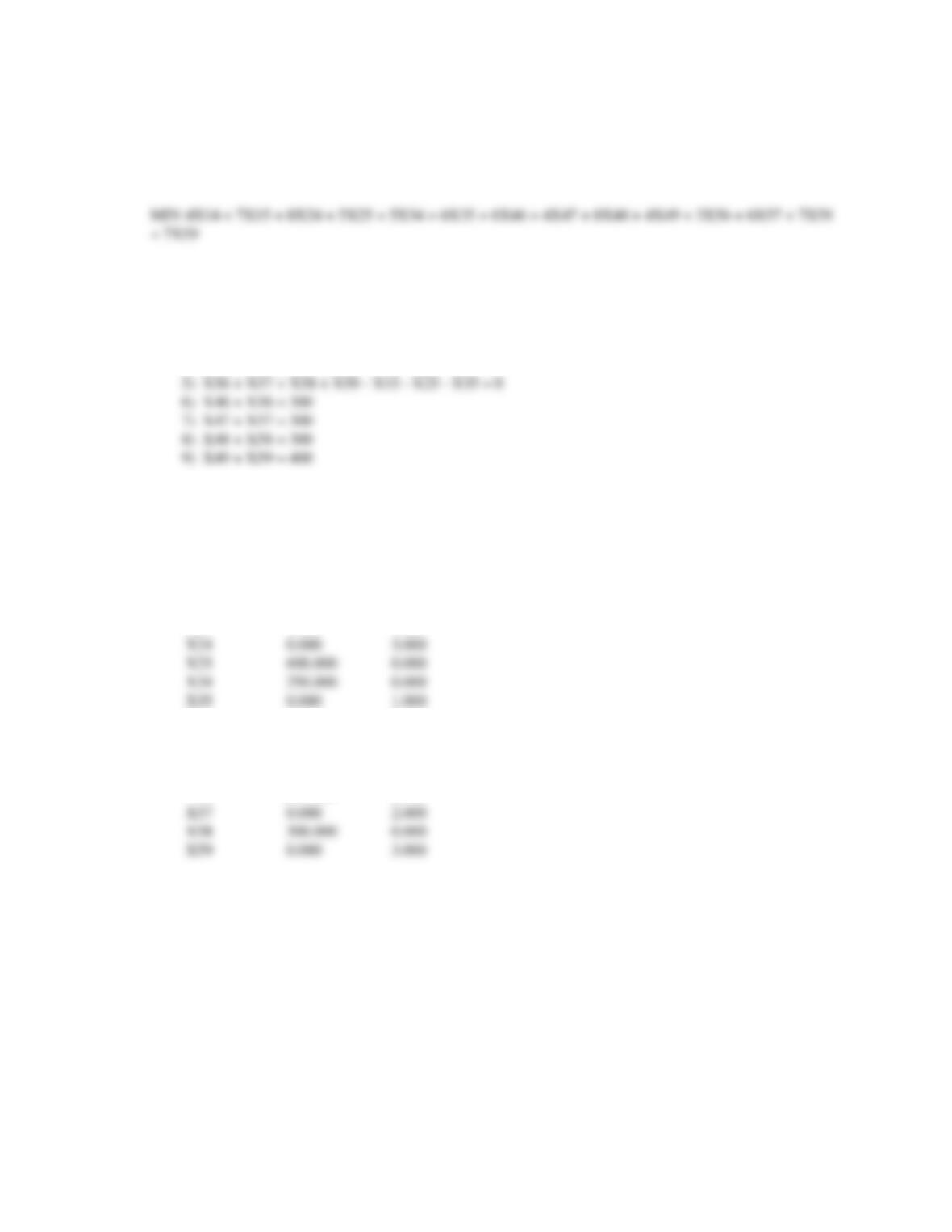
11. a. Network Model
Supplier
1
2
123 4 5 6
614
603
660
639
534
702
680
693
590
693
630
630
1
P1
4
W1
7
C2
6
C1
4
7
6
4
8
Supply
450
Dem and
300
300
Chapter 10
10 – 12
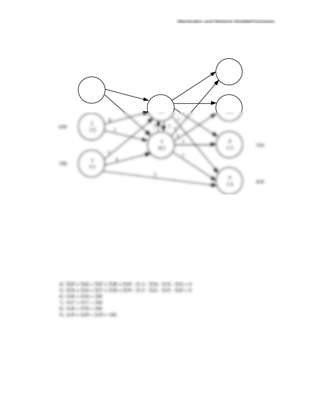
b. & c.
The linear programming formulation and solution is shown below.
LINEAR PROGRAMMING PROBLEM
S.T.
1) X14 + X15 < 450
2) X24 + X25 < 600
3) X34 + X35 < 380
4) X46 + X47 + X48 + X49 – X14 – X24 – X34 = 0
OPTIMAL SOLUTION
Objective Function Value = 11850.000
Variable Value Reduced Costs
————– ————— ——————
X14 450.000 0.000
X46 0.000 3.000
X47 300.000 0.000
X48 0.000 1.000
X49 400.000 0.000
There is an excess capacity of 130 units at plant 3.
10 – 13
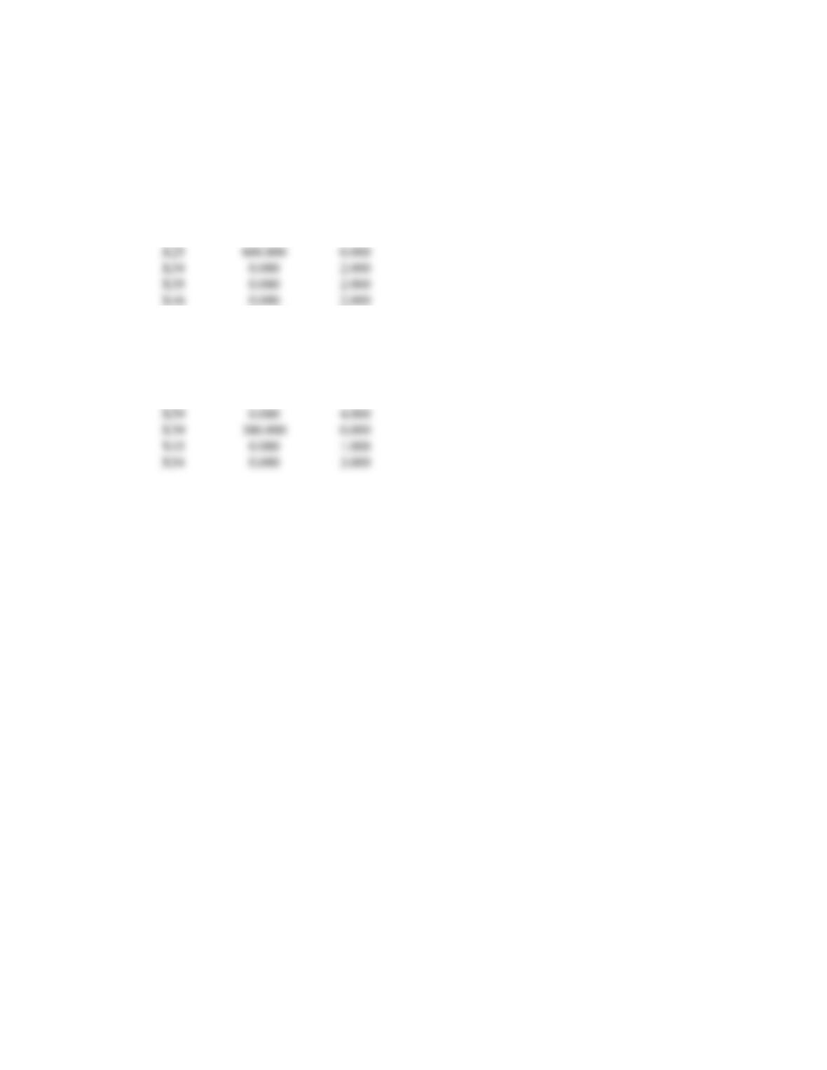
12. a. Three arcs must be added to the network model in problem 23a. The new network is shown.
b.&c.
The linear programming formulation and optimal solution is shown below.
LINEAR PROGRAMMING PROBLEM
MIN 4X14 + 7X15 + 8X24 + 5X25 + 5X34 + 6X35 + 6X46 + 4X47 + 8X48 + 4X49 + 3X56 + 6X57 + 7X58
+ 7X59 + 7X39 + 2X45 + 2X54
S.T.
1) X14 + X15 < 450
2) X24 + X25 < 600
1
P1
4
7
6
C1
4
7
6
4
Supply
450
Dem and
300
300
Chapter 10
10 – 14
OPTIMAL SOLUTION
Objective Function Value = 11220.000
Variable Value Reduced Costs
————– ————— ——————
X14 320.000 0.000
X15 0.000 2.000
X24 0.000 4.000
X47 300.000 0.000
X48 0.000 0.000
X49 20.000 0.000
X56 300.000 0.000
X57 0.000 3.000
X58 300.000 0.000
The value of the solution here is $630 less than the value of the solution for problem 23. The new
shipping route from plant 3 to customer 4 has helped (x39 = 380). There is now excess capacity of
130 units at plant 1.
10 – 15
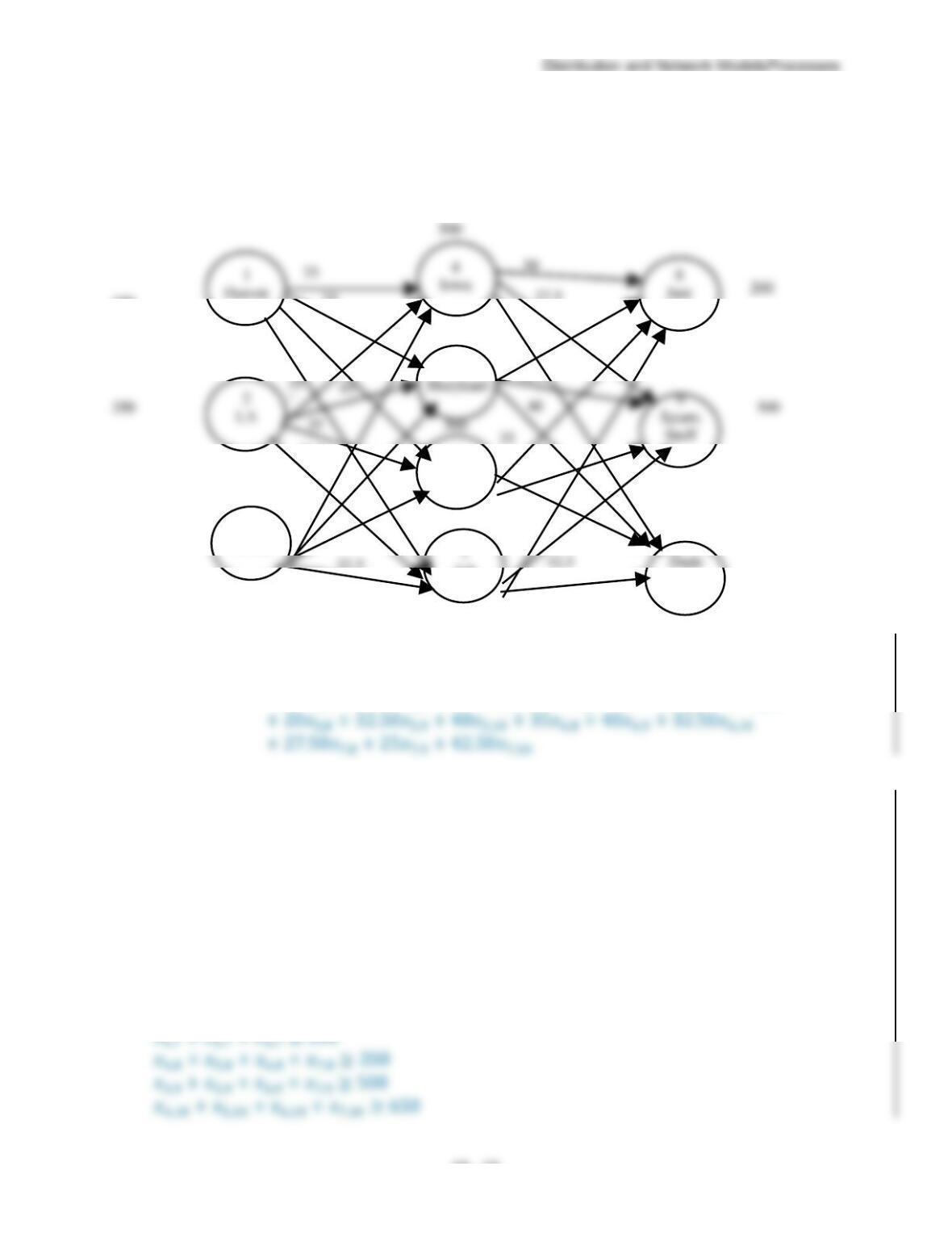
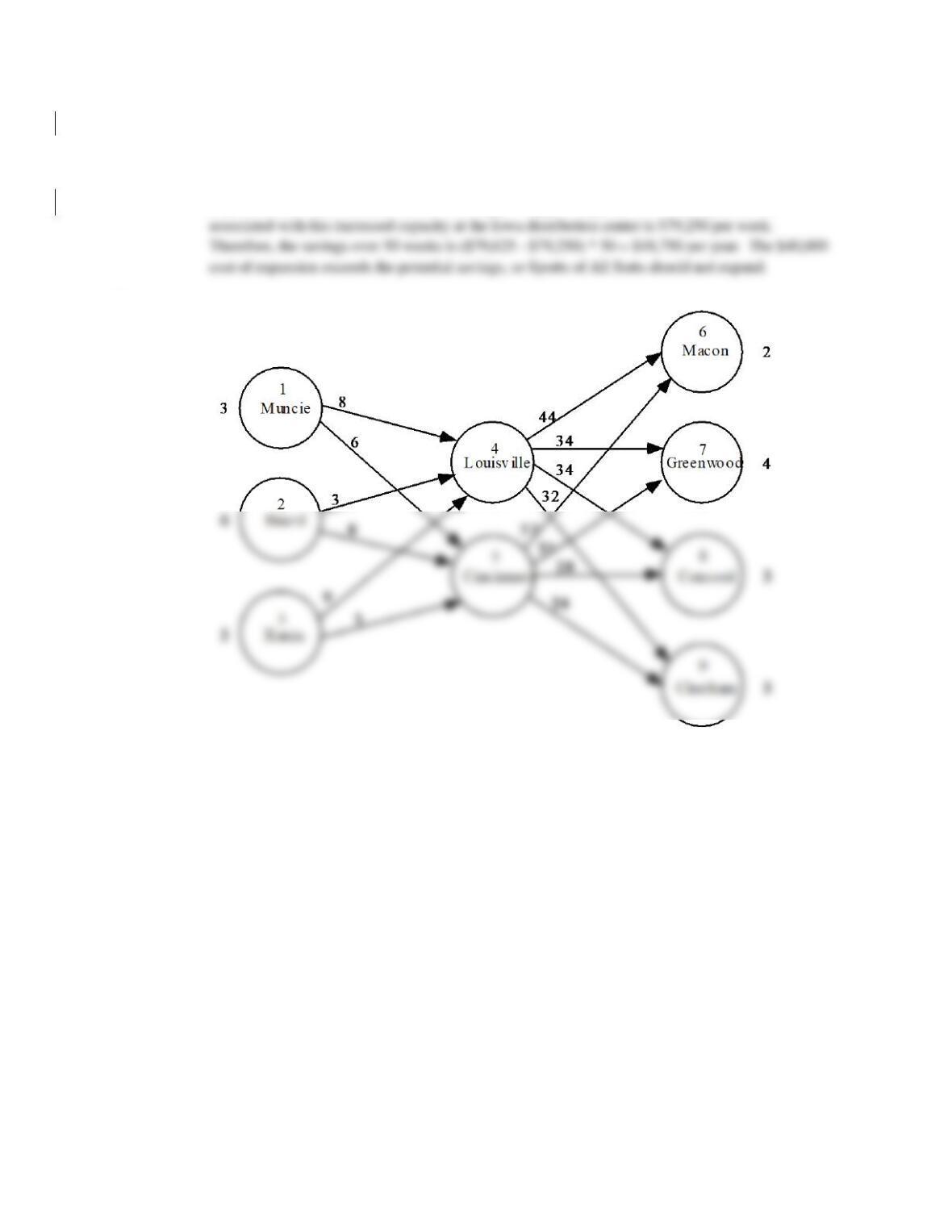
13. a. Network Model
1
4
25
30
200
500
2
45
35
32.5
40
35
500
350
500
42.5
b. Let 𝑥𝑖𝑗 = units shipped from node i to node j
𝑀𝑖𝑛 25𝑥1,4 +25𝑥1,5 +35𝑥1,6 +40𝑥1,7 +35𝑥2,4 +45𝑥2,5 +35𝑥2,6 +42.5𝑥2,7 +40𝑥3,4
+40𝑥3,5 +42.50𝑥3,6 +32.50𝑥3,7 +30𝑥4,8 +27.50𝑦𝑥4,9 +30𝑥4,10
subject to
𝑥1,4 + 𝑥1,5 + 𝑥1,6 + 𝑥1,7 ≤350
𝑥2,4 + 𝑥2,5 + 𝑥2,6 + 𝑥2,7 ≤350
𝑥3,4 + 𝑥3,5 + 𝑥3,6 + 𝑥3,7 ≤700
𝑥1,4 + 𝑥2,4 + 𝑥3,4 = 𝑥4,8 + 𝑥4,9 + 𝑥4,10
𝑥1,5 + 𝑥2,5 + 𝑥3,5 = 𝑥5,8 + 𝑥5,9 + 𝑥5,10
𝑥1,6 + 𝑥2,6 + 𝑥3,6 = 𝑥6,8 + 𝑥6,9 + 𝑥6,10
𝑥1,7 + 𝑥2,7 + 𝑥3,7 = 𝑥7,8 + 𝑥7,9 + 𝑥7,10
𝑥1,4 + 𝑥2,4 + 𝑥3,4 ≤500
𝑥1,5 + 𝑥2,5 + 𝑥3,5 ≤500
𝑥1,6 + 𝑥2,6 + 𝑥3,6 ≤500
3
Austin
10
Sports
Ark
6
Idaho
5
Sports
40
42.5
40
42.5
32.5
25
35
40
20
40
32.5
27.5
25
27.5
30
Demand
Supply
650
350
700
DC Capacity
500
500
Chapter 10
10 – 16
𝑥𝑖𝑗, 𝑦𝑖𝑗 ≥ 0 for all i and j.
Solving the formulation above using Excel Solver we get an optimal cost of $79,625 per week.
c. Replace the seventh constraint above with 𝑥1,4 + 𝑥2,4 + 𝑥3,4 ≤700. The optimal cost
14.
A linear programming model is