
Unadjusted Demand / Seasonal Adjusted
Month Period Demand Forecast Forecast Index Forecast
Jan-18 1 1200 1457 82.3% 81.1% 1182
Feb-18 2 1400 1512 92.6% 91.2% 1379
Mar-18 3 1450 1566 92.6% 91.3% 1429
Apr-18 4 1580 1620 97.5% 96.2% 1558
Apr-19 16 2154 2272 94.8% 96.2% 2185
May-19 17 2430 2326 104.5% 105.9% 2462
Jun-19 18 2827 2380 118.8% 120.2% 2861
Jul-19 19 2877 2435 118.2% 119.4% 2908
Aug-19 20 2687 2489 108.0% 109.0% 2713
Sep-19 21 2492 2543 98.0% 98.9% 2515
SUMMARY OUTPUT
Regression Statistics
Multiple R 0.85
R Square 0.72

Comparing a Two-Period Moving Average and an Exponential Smoothing Model
Two-period moving average model Exponential Smoothing Model
Weight on Period t-2: 0.35 Initial Forecast 65
Weight on Period t-1: 0.65 Alpha (a): 0.3
Period Demand Forecast
Forecast
Error
Absolute
Deviation
Forecast
Forecast
Error
Absolute
Deviation
160 65.00 -5.00 5.00
253 63.50 -10.50 10.50
365 55.45 9.55 9.55 60.35 4.65 4.65
472 60.80 11.20 11.20 61.75 10.26 10.26
572 69.55 2.45 2.45 64.82 7.18 7.18
674 72.00 2.00 2.00 66.98 7.02 7.02

Month Sales (Y) Temp (X) X^2 X*Y b.
a = -767.7
Forecast
b = 98.5
Mar-14 4670 52 2704 242840
Apr-14 5310 58 3364 307980
May-14 6320 69 4761 436080
Jun-14 7080 75 5625 531000
ANSWER:
a.
Using the formula 9-8:
98.5 =
Using the formula 9-9:
=(E17-((C17*B17)/(COUNT(A3:A14))))/(D17-
((C17^2)/(COUNT(A3:A14))))

Month Interest Number of X^2 X*Y
Rate (X) Loans (Y)
17% 20 0.0049 1.4
25% 30 0.0025 1.5
711% 15 0.0121 1.65
89% 20 0.0081 1.8
ANSWER:
a.
a = 41.1454 (intercept term)
b = -259.0308 (regression coefficient for interest rate)

Demand = (35,000 + 4.8 * period) seasonal index
Seasonal Indices
Summer 1.25
Fall 0.90
Winter 0.75
Spring 0.90
ANSWER:
a.

Quarter Demand Forecast Seasonal
Index
Winter 285 250 1.14
Fall 400 400 1.00
ANSWER:
The fall quarter season index is 1.00 so the unadjusted forecast will not be changed when
Month Cheese Cheese Cheese Total
Balls Nachos Potato Sales
Chips
Jan-19 $126,500 $69,000 $34,500 $230,000
Feb-19 $119,600 $73,600 $36,800 $230,000
Mar-19 $115,200 $81,600 $43,200 $240,000
Apr-19 $125,000 $70,000 $55,000 $250,000
May-19 $112,800 $64,800 $62,400 $240,000
Developing product type forecasts from aggregate forecasts in Figure 9.22
and percentages calculated above:
Month Cheese Cheese Cheese Adjusted
Balls Nachos Potato Forecast
Chips
Jan-20 $143,135 $85,872 $57,357 $286,364
Feb-20 $145,547 $87,319 $58,323 $291,189
Mar-20 $147,959 $88,766 $59,290 $296,014

Inches of Average Peak Acre-Feet of
Rainfall Daily Temp, Water Used, Forecast Absolute Absolute %
Year March-June July August Forecast Error Deviation Error MFE =
0
2010 11.7 71.0 31500 29714 1786 1786 0.06
2011 10.0 87.4 35500 46630 -11130 11130 0.31
2012 13.3 91.4 35800 44241 -8441 8441 0.24
2013 8.4 98.3 69700 58697 11003 11003 0.16
SUMMARY OUTPUT
Regression Statistics
Multiple R 0.7048242
R Square 0.4967771
ANOVA
df SS MS F
Significance F
Regression
2779100240.8 389550120.4 5.923147 0.016239
0

Period Actual Forecast Forecast Absolute Absolute % Forecast Forecast Absolute Absolute % Forecast Model 1:
Demand Model 1 Error Deviation Error Model 2 Error Deviation Error MFE = -1
8248 364 -116 116 0.47 486 -238 238 0.96 MAD = 97
9357 280 77 77 0.22 341 16 16 0.04 MAPE = 0.30

Month Demand Forecast Forecast Absolute Absolute % MFE = -5
Error Deviation Error MAD = 44
January 1040 1055 -15 15 0.01 MAPE = 0.04
February 990 1052 -62 62 0.06
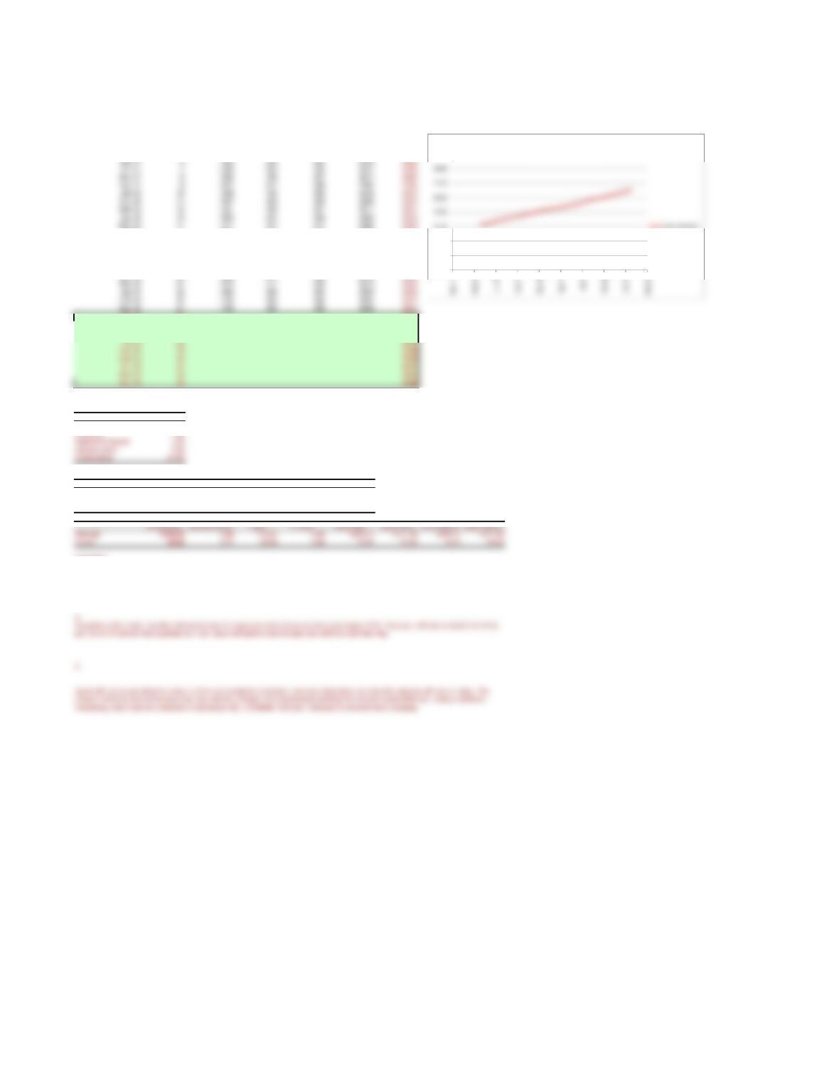
Month Period Bomber Hook King Sir Slice-A-Lot Total demand
Forecast, total
demand
Apr-17 1 1410 377 343 2130 2126
May-17 2 1417 381 344 2142 2146
Jun-17 3 1434 387 346 2167 2167
Jul-17 4 1452 391 349 2192 2187
Aug-17 5 1466 396 350 2212 2208
Jun-18 15 1587 441 375 2403 2413
Jul-18 16 1595 445 377 2417 2433
Aug-18 17 1613 454 381 2448 2454
Sep-18 18 1631 461 384 2476 2474
Oct-18 19 1642 464 386 2492 2495
Nov-18 20 1656 471 389 2516 2515
Apr-19 25 2618
May-19 26 2638
Jun-19 27 2659
SUMMARY OUTPUT
Regression Statistics
Multiple R 1.00
ANOVA
df SS MS F Significance F
Regression 1.00 483513.03 483513.03 9789.53 0.00
Residual 22.00 1086.60 49.39
Total 23.00 484599.63
ANSWER:
1.
The linear regression model fits the sample data extremely well. The R^2 value for the model is .99, indicating that the model explains 99% of the
variance in the dependent variable. Note that we forecasted total demand because it is this value that we are interested in when determining whether
or not Top-Slice needs to expand capacity.
1500
1700
1900
2100
Total demand