First Attempt: 240 seconds
Second Attempt: 180 seconds
a.)
b.)
Attempts Until 50% of First Run: 9 (from Table 6.4)
c.)
$0.50
Capacity
Option
Fixed Cost
Variable Cost
Per Unit of
Output
Max. Output
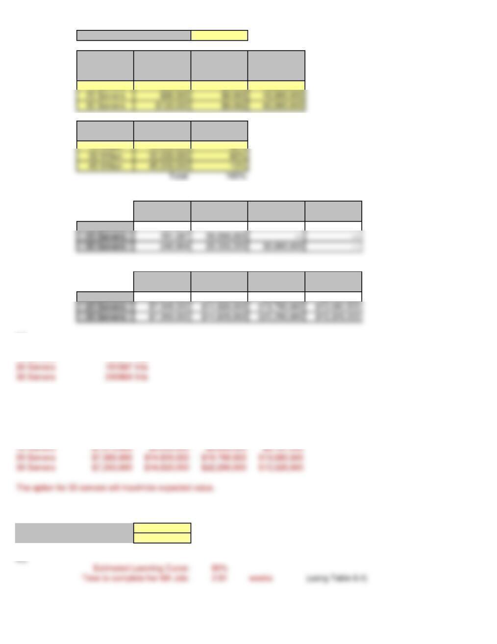
10 Servers $50,000 $0.005 20,000,000
Demand
Scenario
Demand Level Probability
*** Break-Even and Indifference Points ***
Break-Even
Point
10 Servers 20 Servers 30 Servers
10 Servers 101,011 — — —
*** Results for Different Capacity/Demand Combinations ***
15 Million 30 Million 45 Million
Expected
Value
10 Servers $7,375,000 $9,850,000 $9,850,000 $9,107,500
a.)
Break-Even
10 Servers 101011 hits
b.)
Indifference Point between 10 and 20 servers: 20,000,000 hits
c.)
15 Million 30 Million 45 Million Expected Value
First Job: 5 weeks
Second Job: 4 weeks
NOTE: Enter Inputs in Yellow-Shaded Cells.
Revenue per unit of output:
Service Rate: 15 calls per hour
f.)
e.)
Time to finish next 5 jobs (3-7): 15.17 weeks (using Table 6.4)
ong-Run Averages:
Arrival Rate: 11 calls per hour
g.)
h.)
*** Per Job Estimates ***
Revenue: $2,000.00
Cost: Hours Per Hour Total
Labor 30 $10.00 $300.00
Equipment 20 $20.00 $400.00
Total Cost: $700.00
*** Demand Scenario Estimates ***
Demand
Scenario
Demand Level Probability
High 300 30%
*** Capacity Option Estimates ***
Part a)
Capacity
Option
Number of
Labor Hours
Number of
Equipment
Hours
Fixed Cost
Break-Even
Point
Max. Number
of Jobs
Handled
Part b)
*** Per Job Estimates ***
Revenue: $2,000.00
Cost: Hours Per Hour Total
Labor 30 $10.00 $300.00
Equipment 20 $20.00 $400.00
Total Cost: $700.00
*** Demand Scenario Estimates ***
Demand
Scenario
Demand Level Probability
High Demand 300 30%
*** Capacity Option Estimates ***
Capacity
Option
Number of
Labor Hours
Number of
Equipment
Hours
Fixed Cost
Break-Even
Point
Max.
Number of
Jobs
Handled
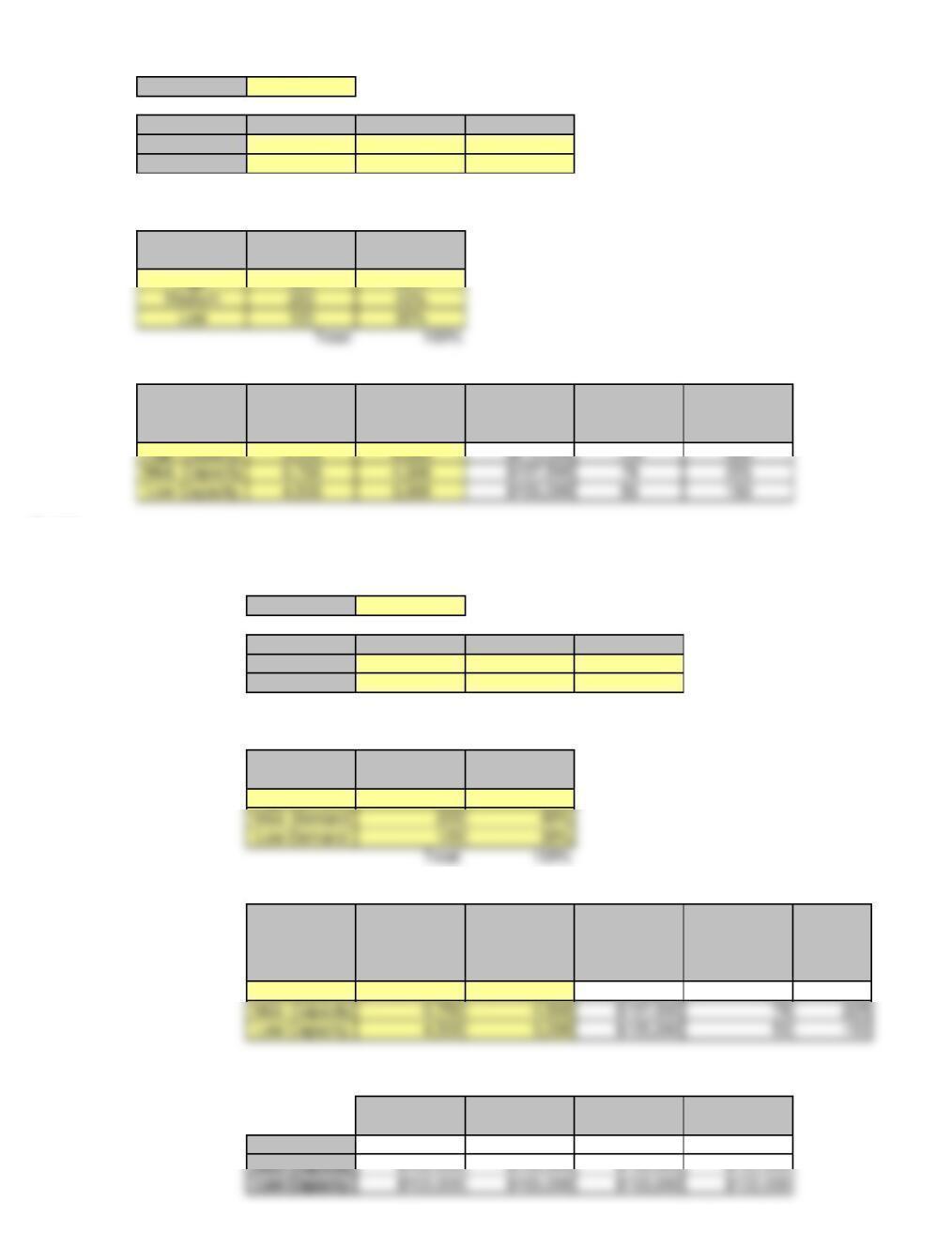
High Capacity 9,000 6,000 $210,000 105 300
*** Results for Different Capacity/Demand Combinations ***
High Demand Med. Demand Low Demand
Expected
Profit
High Capacity $204,000 $204,000 $204,000 $204,000
High Demand Level Probability Profit
NOTE: Enter Inputs in Yellow-Shaded Cells.
NOTE: Enter Inputs in Yellow-Shaded Cells.
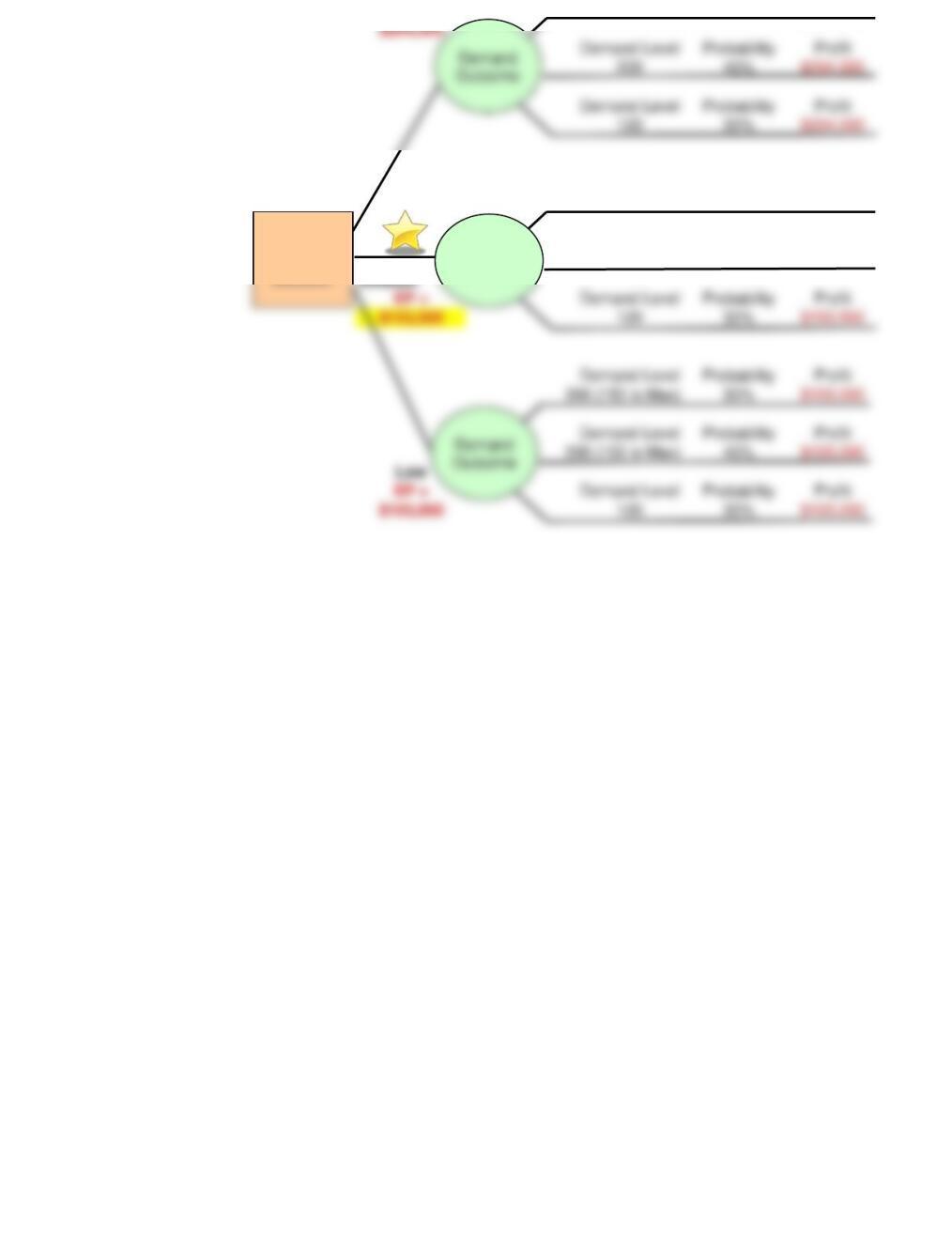
EP = 300 30% $204,000
Demand Level Probability Profit
300 (225 is Max) 30% $153,500
Demand Level Probability Profit
200 40% $153,500
EP = Demand Level Probability Profit
EP = Demand Level Probability Profit
Capacity
Option
Decision
Demand
Outcome
$100.00
Capacity
Option
Fixed Cost
Variable Cost
Per Unit of
Output
Max. Output
Option A $0.00 $30.00 200
Demand
Scenario
Demand Level Probability
Low 125 25%
*** Break-Even and Indifference Points ***
Break-Even
Point
Option A Option B Option C
Option A 0.00 — — —
*** Results for Different Capacity/Demand Combinations ***
Low Medium High
Expected
Value
Option A $8,750.00 $14,000.00 $14,000.00 $12,687.50
NOTE: Enter Inputs in Yellow-Shaded Cells.
Revenue per unit of output:
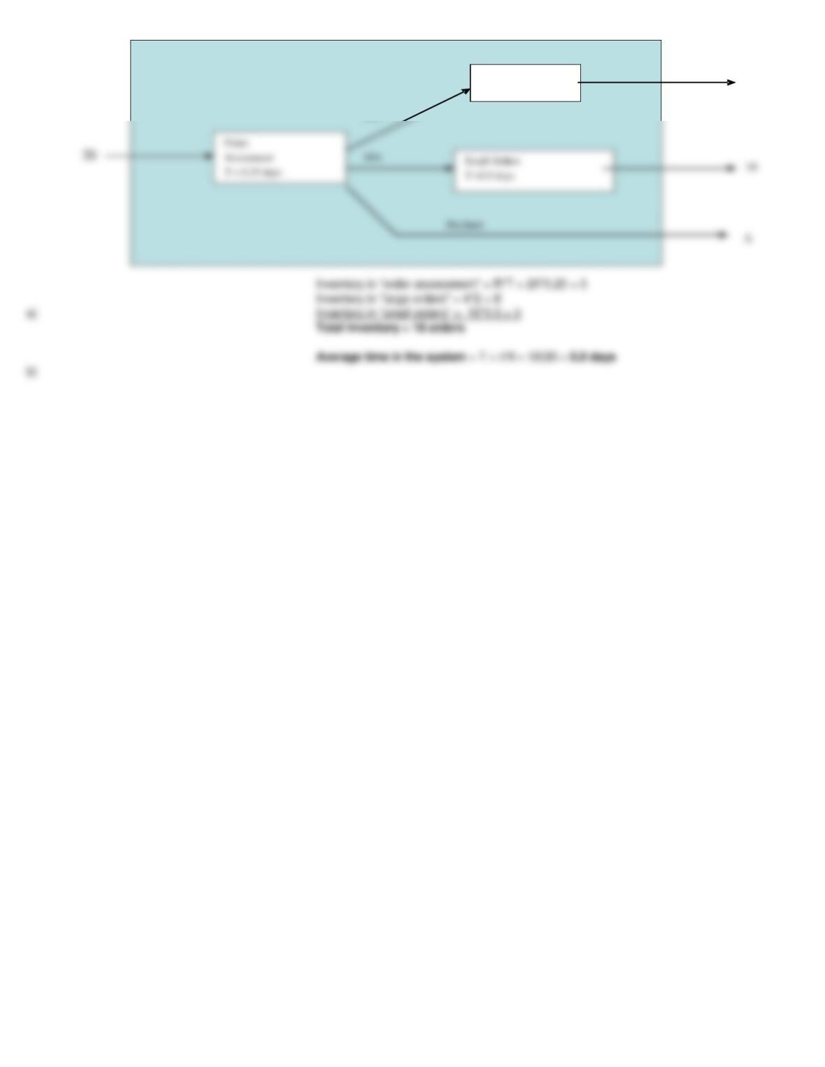
Large Orders
T = 2 days
20%
4
$7.00
$2.90
Capacity
Option
Fixed Cost
Variable Cost
Per Unit of
Output
Max. Output
No Roaster $0.00 $3.00 14,400
Total: 100%
*** Break-Even and Indifference Points ***
Break-Even
Point
Indifference
Point
No Roaster 0 —
Question 1.)
NOTE: Enter Inputs in Yellow-Shaded Cells.
Revenue per unit of output (first 14,400 lbs):
Revenue per unit of output (after 14,400 lbs):
The two capacity options that Robbie needs to consider are buying vs. not buying a coffee roaster. The costs of not
buying a roaster are $0.00 (Fixed) and $3.00 (Variable) while the costs of buying a roaster are $35,000 (Fixed) and
Demand
Demand Level Probability
18,000 33%
Demand Level Probability
25,000 33%
Question 2.)
Question 3.)
Question 4.)
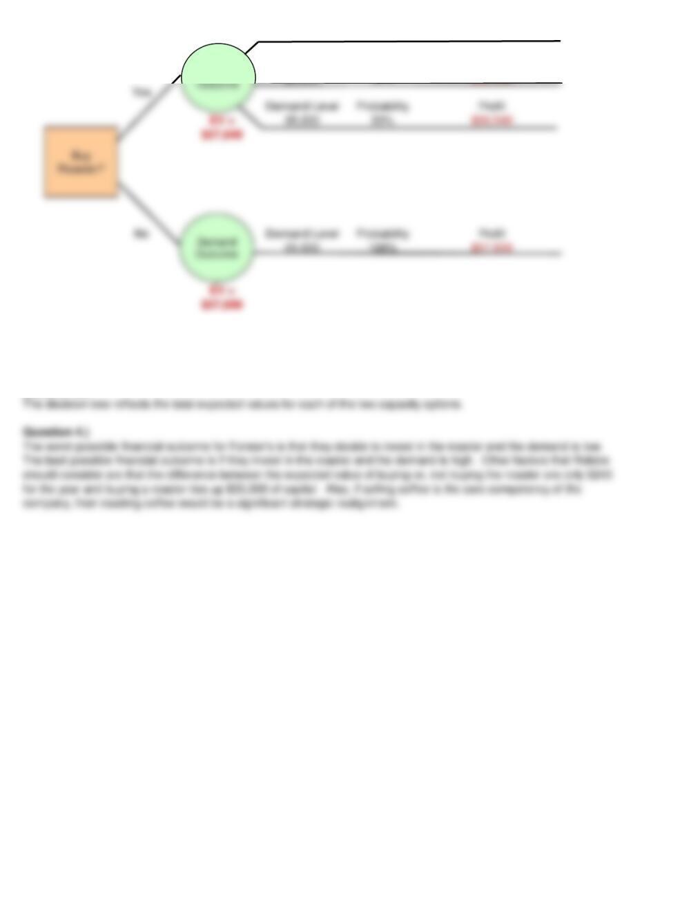
The demand scenarios do not make a difference in the expected profit if Forster’s does not invest in the roaster since
all of the demand scenarios are greater than the 14,400 maximum that Forster’s will sell in-house.
Profit
$47,440
Expected Value
$56,540
Demand
Profit
$57,600
$69,540
Profit