MODULE 7
Linear Programming: The Simplex Method
TEACHING SUGGESTIONS
Teaching Suggestion M7.1: Meaning of Slack Variables.
Slack variables have an important physical interpretation and represent a valuable commodity,
such as unused labor, machine time, money, space, and so forth.
Teaching Suggestion M7.2: Initial Solutions to LP Problems.
Explain that all initial solutions begin with X1 = 0, X2 = 0 (that is, the real variables set to zero),
Teaching Suggestion M7.3: Substitution Rates in a Simplex Tableau.
Perhaps the most confusing pieces of information to interpret in a simplex tableau are “substitu-
Teaching Suggestion M7.4: Hand Calculations in a Simplex Tableau.
It is almost impossible to walk through even a small simplex problem (two variables, two con-
straints) without making at least one arithmetic error. This can be maddening for students who
know what the correct solution should be but can’t reach it. We suggest two tips:
Teaching Suggestion M7.5: Infeasibility Is a Major Problem in Large LP Problems.
As we noted in Teaching Suggestion 7.6, students should be aware that infeasibility commonly
ALTERNATIVE EXAMPLES
Alternative Example M7.1: Simplex Solution to Alternative Example 7.1 (see Chapter 7 of
Solutions Manual for formulation and graphical solution).
1st Iteration
Cj→
Solution
Mix
3
9
0
0
Quantity
X1
X2
S1
S2
2nd Iteration
Cj→
Solution
Mix
3
9
0
0
Quantity
X1
X2
S1
S2
9
X2
14
1
14
0
6
0
S2
12
−12
9
0
0
−94
0
0
1
4
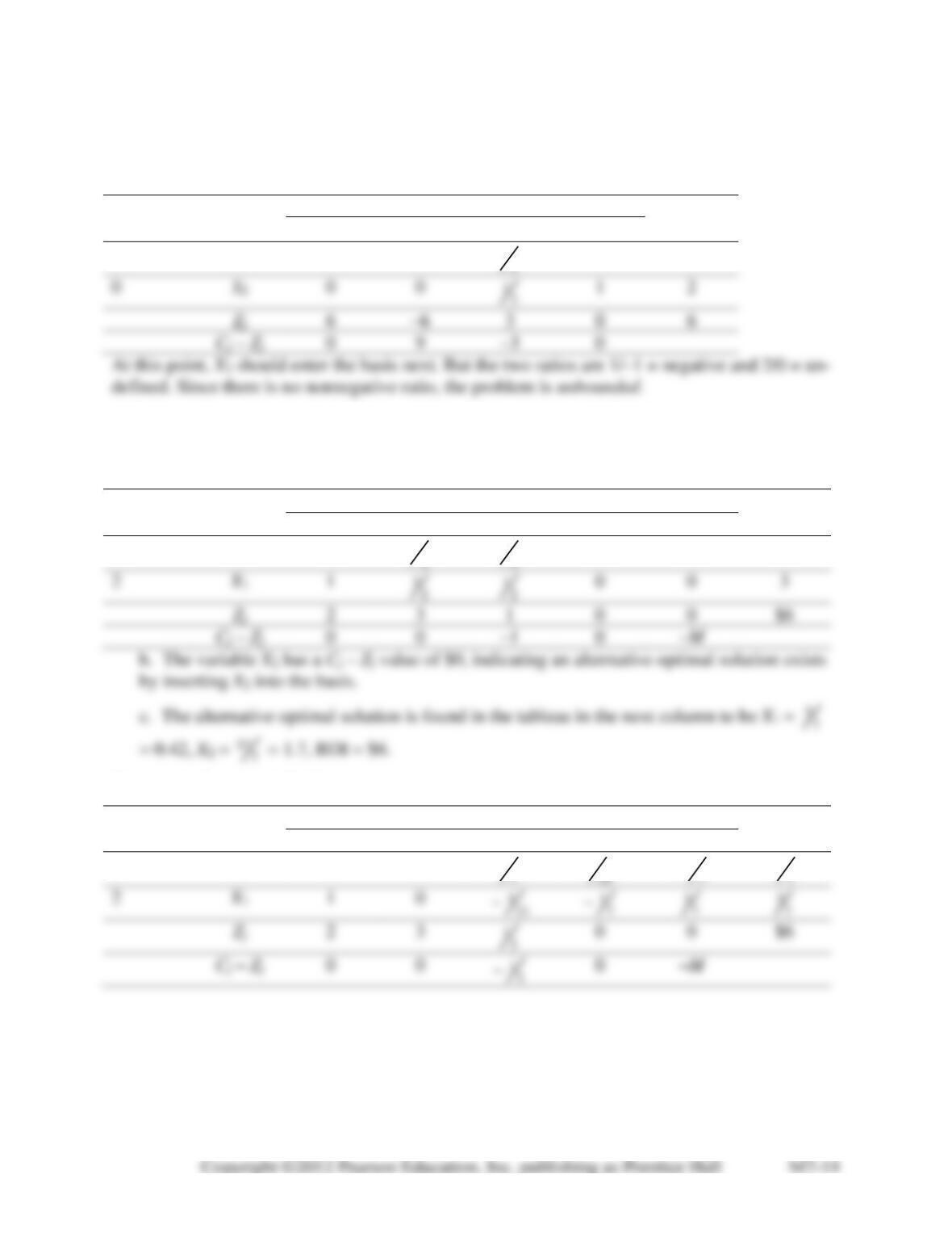
This is not an optimum solution since the X1 column contains a positive value. More profit re-
mains ($
34
per #1).
3rd/Final Iteration
Cj→
Solution
Mix
3
9
0
0
Quantity
X1
X2
S1
S2
9
X2
0
1
12
−12
4
3
X1
1
0
−1
2
8
3
9
0
0
−32
−32
Alternative Example M7.2: Set up an initial simplex tableau, given the following two con-
straints and objective function:
Minimize Z = 8X1 + 6X2
The constraints and objective function may be rewritten as:
Minimize = 8X1 + 6X2 + 0S1 + 0S2 + MA1 + MA2
2X1 + 4X2 – 1S1 + 0S2 + 1A1 + 0A2 = 8
3X1 + 2X2 + 0S1 – 1S2 + 0A1 + 1A2 = 6
The first tableau would be:
Cj→
Solution
Mix
8
6
0
0
M
M
Quantity
X1
X2
S1
S2
A1
A2
M
A1
2
4
–1
0
1
0
8
M
A2
3
2
0
–1
0
1
6
M
M
M
M
0
0
The second tableau:
Cj→
Solution
Mix
8
6
0
0
M
M
Quantity
X1
X2
S1
S2
A1
A2
6
X2
12
1
−14
0
14
0
2
A2
12
−12
3 + 2M
−32+12
32−12
−32+32
The third and final tableau:
Cj→
Solution
Mix
8
6
0
0
M
M
Quantity
X1
X2
S1
S2
A1
A2
6
X2
0
1
−38
14
−14
8
X1
1
0
14
−12
−14
12
8
6
−14
−52
14
0
0
14
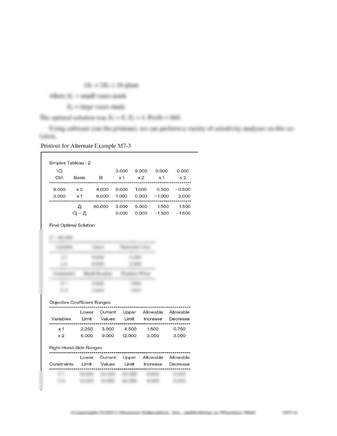
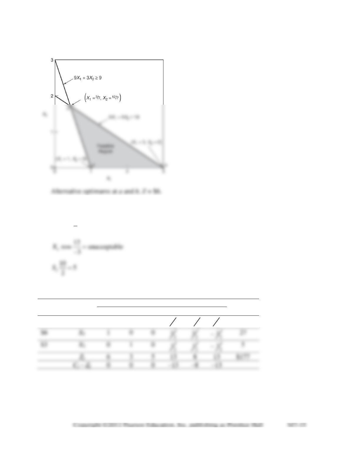
Alternative Example M7.3: Referring back to Hal, in Alternative Example 7.1, we had a for-
mulation of:
Maximize Profit = $3X1 + $9X2
Subject to: 1X1 + 4X2 24 clay
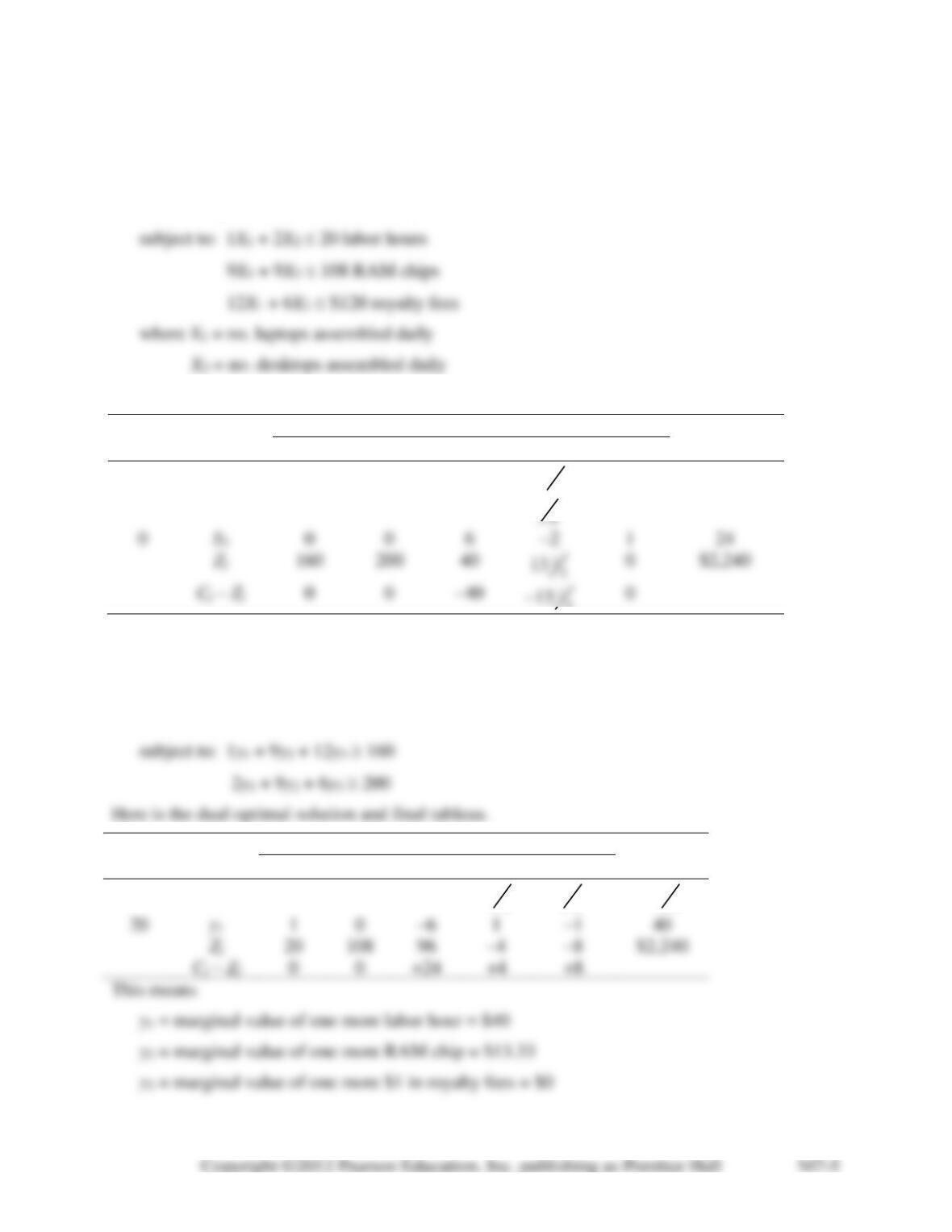
Alternative Example M7.4: Levine Micros assembles both laptop and desktop personal com-
puters. Each laptop yields $160 in profit; each desktop $200.
The firm’s LP primal is:
Maximize profit = $160X1 + $200X2
Here is the primal optimal solution and final simplex tableau.
Cj→
Solution
Mix
$160
$200
0
0
0
Quantity
X1
X2
S1
S2
S3
200
X2
0
1
1
−19
0
8
160
X1
1
0
–1
13 13
0
0
0
0
0
4
−13 13
or X1 = 4, X2 = 8, S3 = $24 in slack royalty fees paid
Profit = $2,240/day
Here is the dual formulation:
Minimize Z = 20y1 + 108y2 + 120y3
Cj→
Solution
Mix
20
108
120
0
0
Quantity
y1
y2
y3
S1
S2
108
y2
0
1
2
13 13
SOLUTIONS TO DISCUSSION QUESTIONS AND PROBLEMS
M7-1. The purpose of the simplex method is to find the optimal solution to LP problems in a
systematic and efficient manner. The procedures are described in detail in Section M7.6.
M7-2. Differences between graphical and simplex methods: (1) Graphical method can be used
only when two variables are in model; simplex can handle any dimensions. (2) Graphical method
must evaluate all corner points (if the corner point method is used); simplex checks a lesser
M7-3. Slack variables convert constraints into equalities for the simplex table. They represent
a quantity of unused resource and have a zero coefficient in the objective function.
M7-4. The number of basic variables (i.e., variables in the solution) is always equal to the num-
ber of constraints. So in this case there will be eight basic variables. A nonbasic variable is one
M7-5. Pivot column: Select the variable column with the largest positive Cj – Zj value (in a max-
imization problem) or smallest negative Cj – Zj value (in a minimization problem).
M7-6. Maximization and minimization problems are quite similar in the application of the sim-
plex method. Minimization problems usually include constraints necessitating artificial and sur-
M7-7. The Zj values indicate the opportunity cost of bringing one unit of a variable into the so-
lution mix.
M7-8. The Cj – Zj value is the net change in the value of the objective function that would result
from bringing one unit of the corresponding variable into the solution.
M7-9. The minimum ratio criterion used to select the pivot row at each iteration is important
M7-10. The variable with the largest objective function coefficient should enter as the first deci-
M7-11. If an artificial variable is in the final solution, the problem is infeasible. The person for-
mulating the problem should look for the cause, usually conflicting constraints.
M7-12. An optimal solution will still be reached if any positive Cj – Zj value is chosen. This
M7-13. A shadow price is the value of one additional unit of a scarce resource. The solutions to
M7-14. The dual will have 8 constraints and 12 variables.
M7-15. The right-hand-side values in the primal become the dual’s objective function coeffi-
cients.
M7-16. The student is to write his or her own LP primal problem of the form:
maximize profit = C1X1 + C2X2
subject to A11X1 + A12X2 B1
A21X1 + A22X2 B2
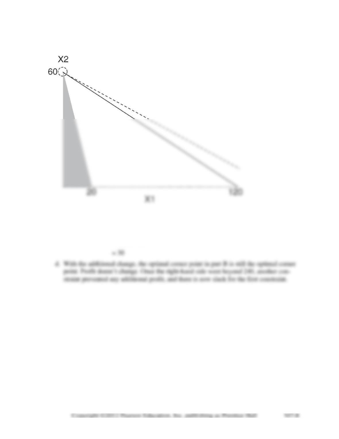
M7-17. a.
b. The new optimal corner point is (0,60) and the profit is 7,200.
c. The shadow price = (increase in profit)/(increase in right-hand side value)
= (7,200 – 2,400)/(240 – 80)
= 4,800/160
M7-18. a. See the table below.
Table for Problem M7-18
Cj→
Solution
Mix
$900
$1,500
$0
$0
Quantity
X1
X2
S1
S2
b. 14X1 + 4X2 3,360
10X1 + 12X2 9,600
X1, X2 0
c. Maximize profit = 900X1 + 1,500X2
d. Basis is S1 = 3,360, S2 = 9,600.
M7-19. a. Maximize earnings = 0.8X1 + 0.4X2 + 1.2X3 – 0.1X4 + 0S1 + 0S2 – MA1 – MA2
subject to
X1 + 2X2 + X3 + 5X4 + S1 = 150
Table for Problem M7-19b
c. S1 = 150, A1 = 70, A2 = 120, all other variables = 0
Cj→
Solution
Mix
0.8
0.4
1.2
−0.1
0
0
−M
−M
Quantity
X1
X2
X3
X4
S1
S2
A1
A2
0
S1
1
2
1
5
1
0
0
0
150
0
1
8
0
0
1
0
6
7
2
0
0
1
120
0
0
0
0
M7-20. First tableau:
Cj→
Solution
Mix
$3
$5
$0
$0
Quantity
X1
X2
S1
S2
$0
S1
0
1
1
0
6
Second tableau:
Cj→
Solution
Mix
$3
$5
$0
$0
Quantity
X1
X2
S1
S2
$5
X2
0
1
1
0
6
$0
3
0
1
6
Third and optimal tableau:
Cj→
Solution
Mix
$3
$5
$0
$0
Quantity
X1
X2
S1
S2
$5
X2
0
1
1
0
6
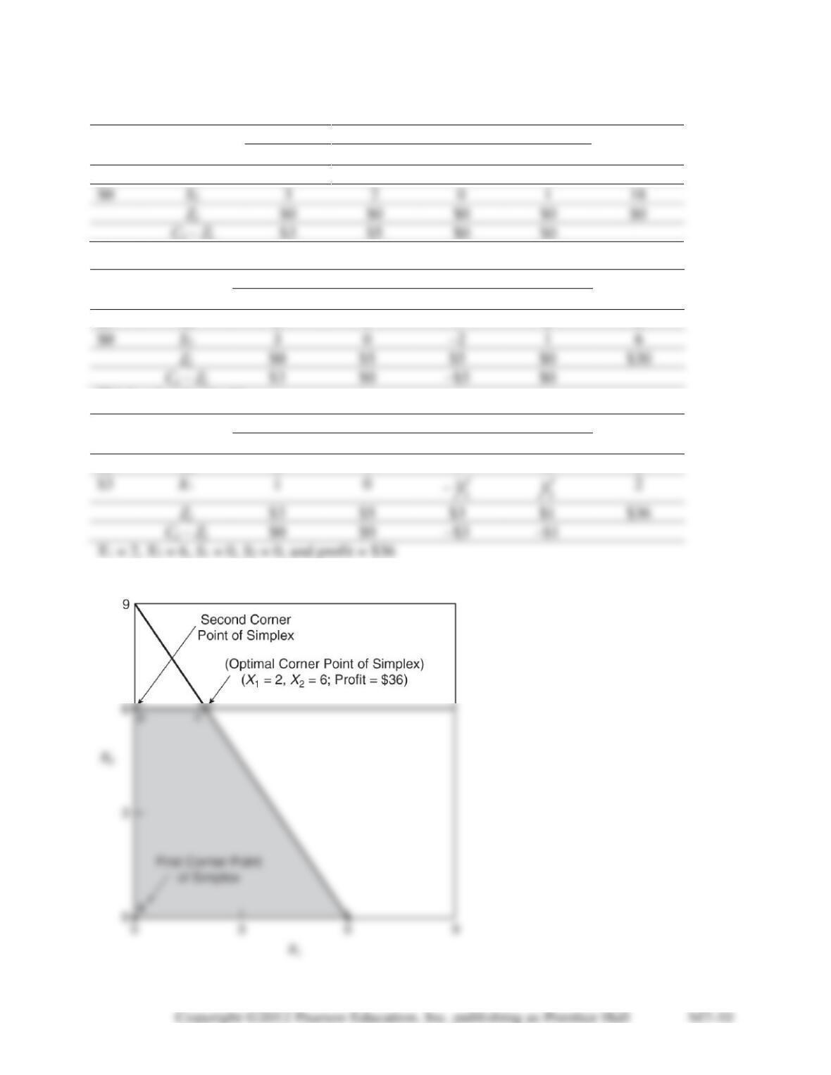
Graphical solution to Problem M7-20:
M7-21. a.
b.
Cj→
Solution
Mix
10
8
0
0
Quantity
X1
X2
S1
S2
0
S1
4
2
1
0
80
0
S2
1
2
0
1
50
0
0
0
0
0
8
0
0
This represents the corner point (0,0).
c. The pivot column is the X1 column. The entering variable is X1.
d. Ratios: Row 1: 80/4 = 20
Row 2: 50/1 = 50
These represent the points (20,0) and (50,0) on the graph.
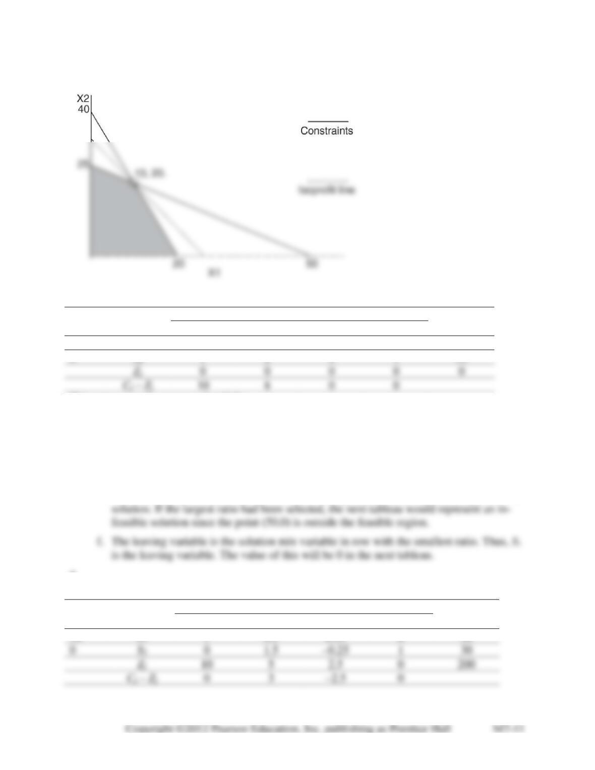
e. The smallest ratio is 20, so 20 units of the entering variable (X1) will be brought into the
g.
Second iteration
Cj→
Solution
Mix
10
8
0
0
Quantity
X1
X2
S1
S2
10
X1
1
0.5
0.25
0
20
0
S2
0
1.5
1
30
5
0

Third iteration
Cj→
Solution
Mix
10
8
0
0
Quantity
X1
X2
S1
S2
10
X1
1
0
0.3333
–0.3333
10
8
X2
0
1
–0.1667
0.6667
20
8
0
0
h. The second iteration represents the corner point (20,0). The third (and final) iteration repre-
sents the point (10,20).
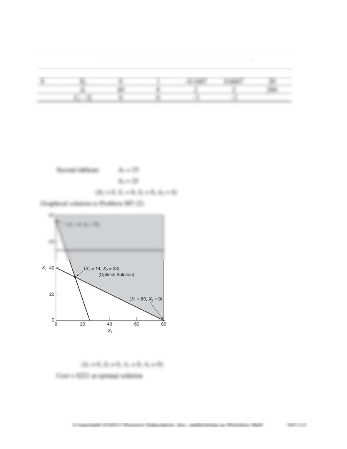
M7-22. Basis for first tableau: A1 = 80
A2 = 75
(X1 = 0, X2 = 0, S1 = 0, S2 = 0)
Third tableau: X1 = 14
X2 = 33
M7-23. This problem is infeasible. All Cj – Zj are zero or negative, but an artificial variable re-
mains in the basis.
M7-24. At the second iteration, the following simplex tableau is found:
Cj→
Solution
Mix
6
3
0
0
Quantity
X1
X2
S1
S2
6
X1
1
–1
0
S2
0
0
1
2
0
1
M7-25. a. The optimal solution using simplex is X1 = 3, X2 = 0. ROI = $6. This is illustrated in
the problem’s final simplex tableau:
Tableau for Problem M7-25a
Cj→
Solution
Mix
2
3
0
0
−M
Quantity
X1
X2
S1
S2
A1
0
S1
0
2
X1
1
0
0
3
1
–1
6
Tableau for Problem M7-25c
Cj→
Solution
Mix
2
3
0
0
−M
Quantity
X1
X2
S1
S2
A1
3
X2
0
1
2
3
0
0
0
0
0
12 7
d. The graphical solution is shown below.
M7-26. This problem is degenerate. Variable X2 should enter the solution next. But the ratios are
as follows:
3
5
row 5
1
X=
Since X3 and S2 are tied, we can select one at random, in this case S2. The optimal solution is
shown below. It is X1 = 27, X2 = 5, X3 = 0, profit = $177.
Cj→
Solution
Mix
6
3
5
0
0
0
Quantity
X1
X2
X3
S1
S2
S3
$5
X3
0
0
1
$6
X1
1
0
0
$3
X2
0
1
0
5
0
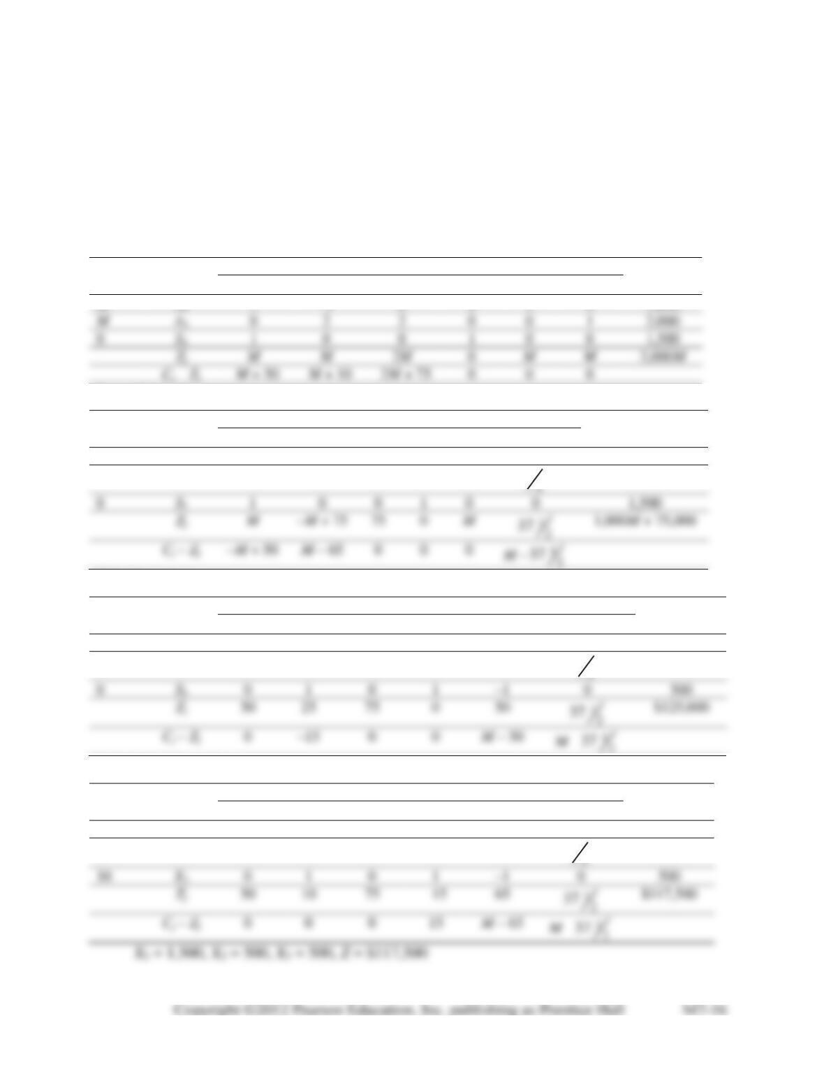
M7-27. Minimum cost = 50X1 + 10X2 + 75X3 + 0S1 + MA1 + MA2
subject to
1X1 – 1X2 + 0X3 + 0S1 + 1A1 + 0A2 = 1,000
0X1 + 2X2 + 2X3 + 0S1 + 0A1 + 1A2 = 2,000
1X1 + 0X2 + 0X3 + 1S1 + 0A1 + 0A2 = 1,500
First iteration:
Cj→
Solution
Mix
50
10
75
0
M
M
Quantity
X1
X2
X3
S1
A1
A2
M
A1
1
–1
0
0
1
0
1,000
A2
0
2
0
1
0
1
0
0
1
0
0
1,500
M
M
0
0
0
Second iteration:
Cj→
Solution
Mix
50
10
75
0
M
M
Quantity
X1
X2
X3
S1
A1
A2
M
A1
1
–1
0
0
1
0
1,000
75
X3
0
1
1
0
0
0
S1
0
1,000
Third iteration:
Cj→
Solution
Mix
50
10
75
0
M
M
Quantity
X1
X2
X3
S1
A1
A2
50
X1
1
–1
0
0
1
0
1,000
75
X3
0
1
1
0
0
0
S1
0
1
0
1
75
0
50
$125,000
0
0
0
1,000
Fourth and final iteration:
Cj→
Solution
Mix
50
10
75
0
M
M
Quantity
X1
X2
X3
S1
A1
A2
50
X1
1
0
0
1
0
0
1,500
75
X3
0
0
1
–1
1
10
X2
0
1
0
1
0
75
65
$117,500
500
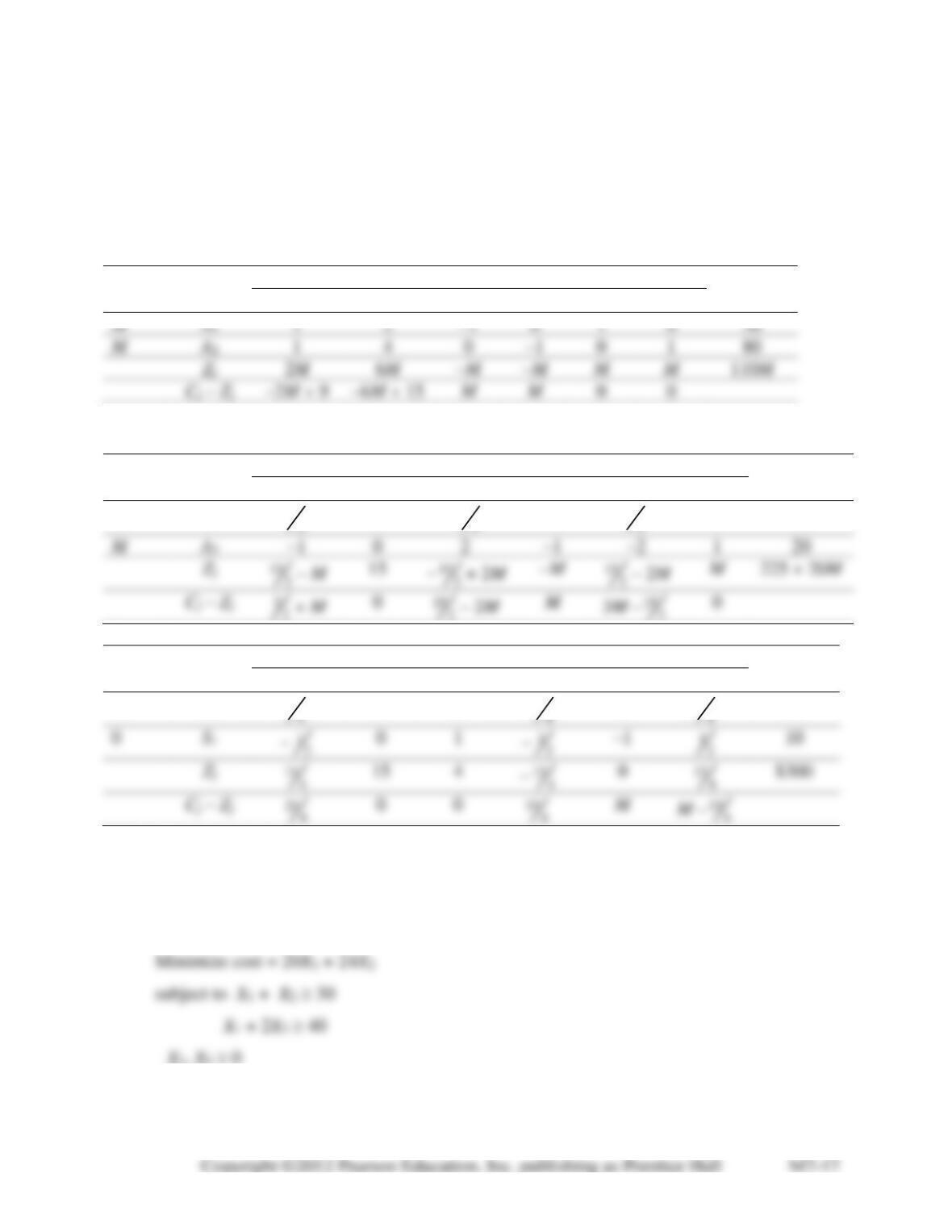
M7-28. X1 = number of kilograms of brand A added to each batch
X2 = number of kilograms of brand B added to each batch
Minimize costs = 9X1 + 15X2 + 0S1 + 0S2 + MA1 + MA2
subject to X1 + 2X2 – S1 + A1 = 30
X1 + 4X2 – S2 + A2 = 80
Cj→
Solution
Mix
$9
$15
$0
$0
M
M
Quantity
X1
X2
S1
S2
A1
A2
First iteration:
Cj→
Solution
Mix
$9
$15
$0
$0
M
M
Quantity
X1
X2
S1
S2
A1
A2
15
X2
0
0
1
0
0
15
32
Second iteration:
Cj→
Solution
Mix
$9
$15
$0
$0
M
M
Quantity
X1
X2
S1
S2
A1
A2
15
X2
0
0
1
10
4
0
$300
0
0
1
0
0
20
214
Third and final iteration:
X1 = 0 kg, X2 = 20 kg, cost = $300
M7-29. X1 = number of mattresses
X2 = number of box springs