MODULE 3
Decision Theory and the Normal Distribution
TEACHING SUGGESTIONS
Teaching Suggestion M3.1: Reviewing the Normal Curve.
Most of the material in this supplement requires the use of the normal curve. A review of the
basic principles of the normal curve found in the probability chapter (Chapter 2) would be help-
ful before this module is started.
Teaching Suggestion M3.2: Covering Break-Even Analysis First.
Covering break-even calculations first helps students get into decision theory and normal curve
Teaching Suggestion M3.3: Spending More Time on EVPI and the Normal Distribution.
EVPI and the normal distribution concepts are difficult for many students. You may need to
SOLUTIONS TO QUESTIONS AND PROBLEMS
M3-1. The purpose of break-even analysis is to help a manager determine at what point overall
M3-2. The normal distribution can be used in break-even analysis when sales are symmetrical
M3-3. The relationship between EMV and the state of nature must be linear when you use the
computations presented in Equation M3-3 in determining EMV from the mean and the standard
deviation. When this relationship is not linear, the approach used in computing EMV cannot be
used.
M3-4. When EVPI is to be computed using a state of nature that follows a normal distribution,
three steps are required. The first step is to determine the opportunity loss function. The second
M3-5.
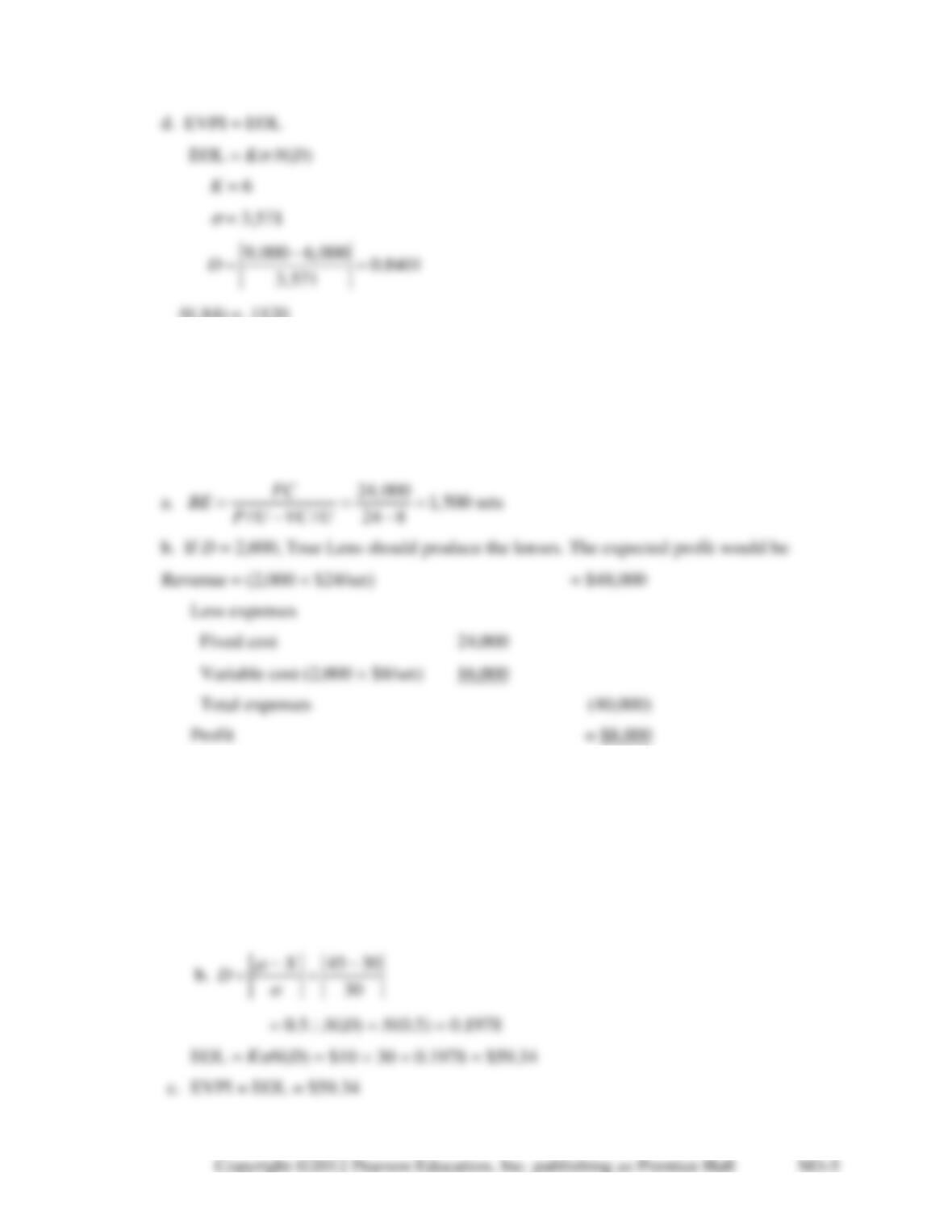
M3-6. a. OLF = K(BE – X) for X BE
OLF = 0 for X BE
with
K = $8
= 10,000
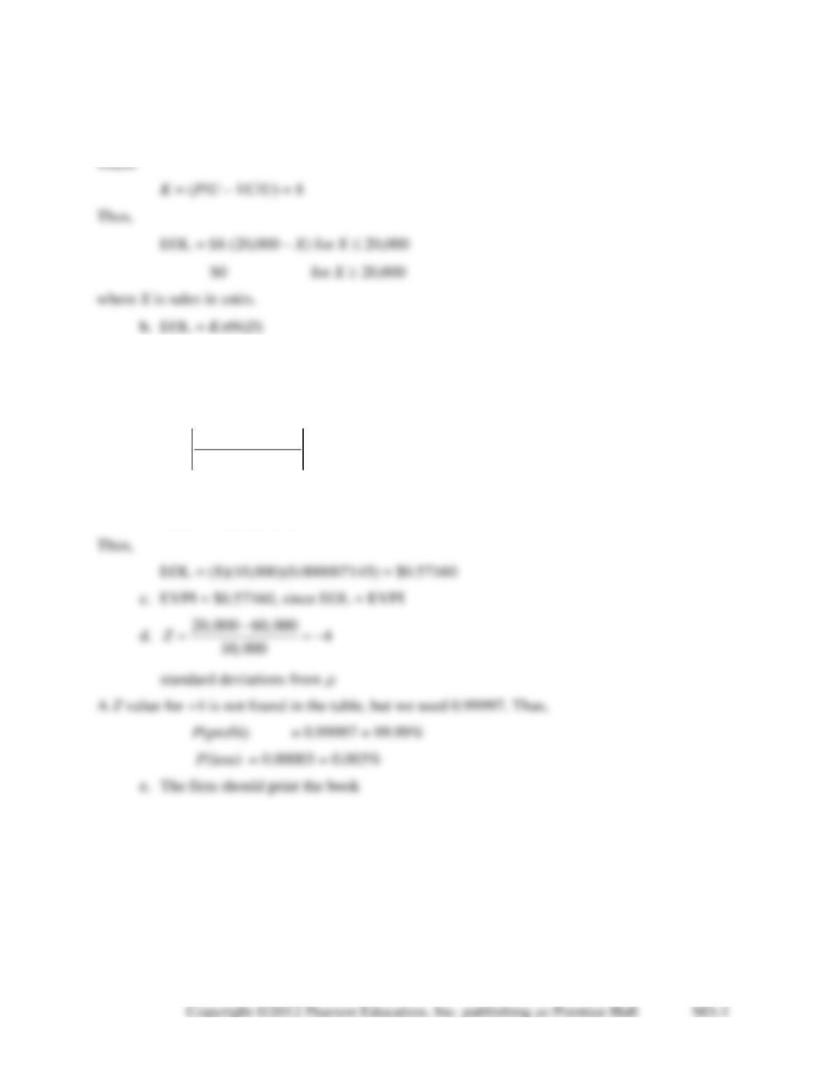
60,000 20,000 4
10,000
D−
==
and
N(D) = 0.000007145.
M3-7.
a.
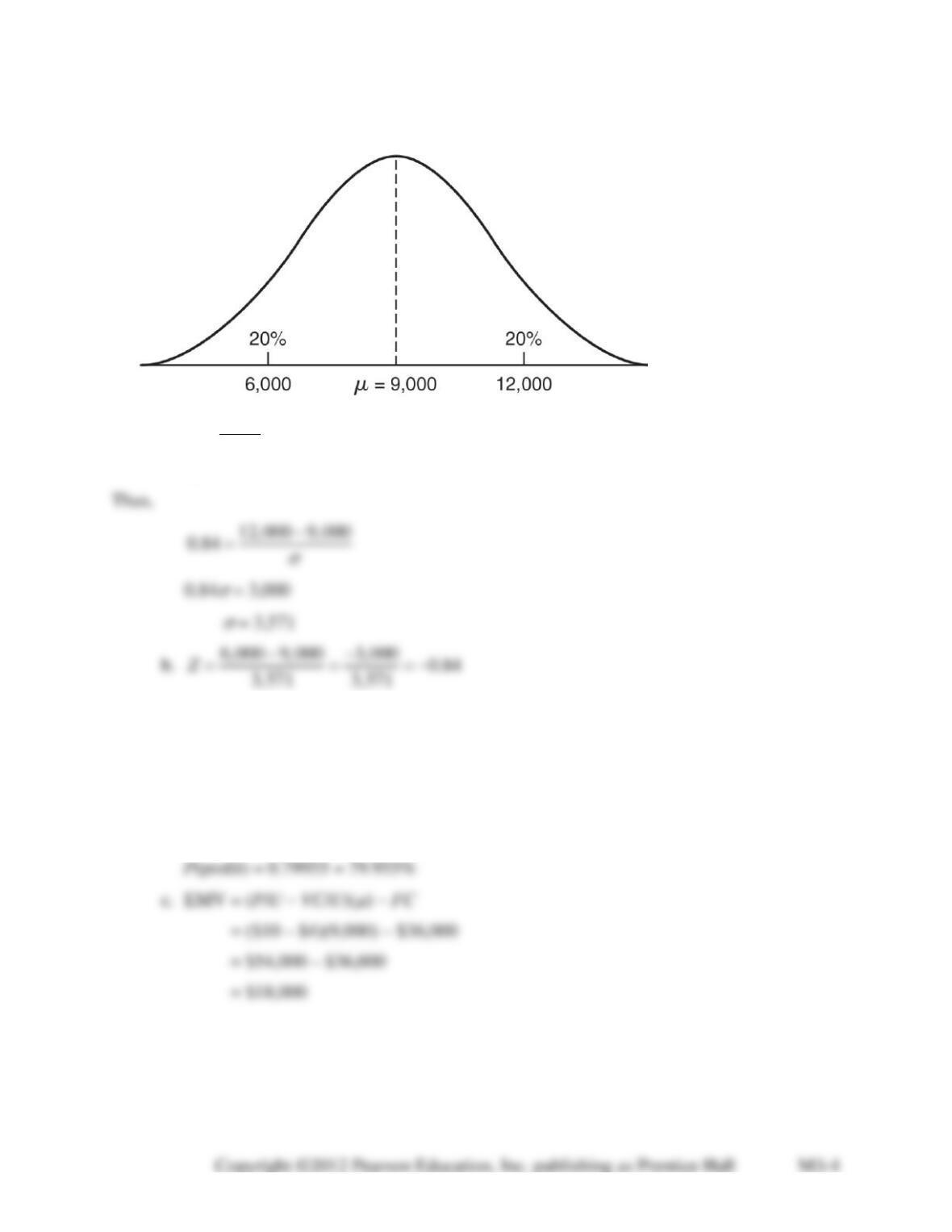
d
Z
−
=
(area to the left of 12,000 = 0.80; from Appendix A, Z value for 0.80 =
0.84)
Using Appendix A gives
Z(0.84) = 0.79955
1 – 0.79955 = 0.20045
Thus,
P(loss) = 0.20045 = 20.045%
N(.84) = .1120
Thus, EOL = (6)(3571)(0.1120) = $2,399.71, and Rudy should be willing to pay up to $2,399.71
for a marketing research study.
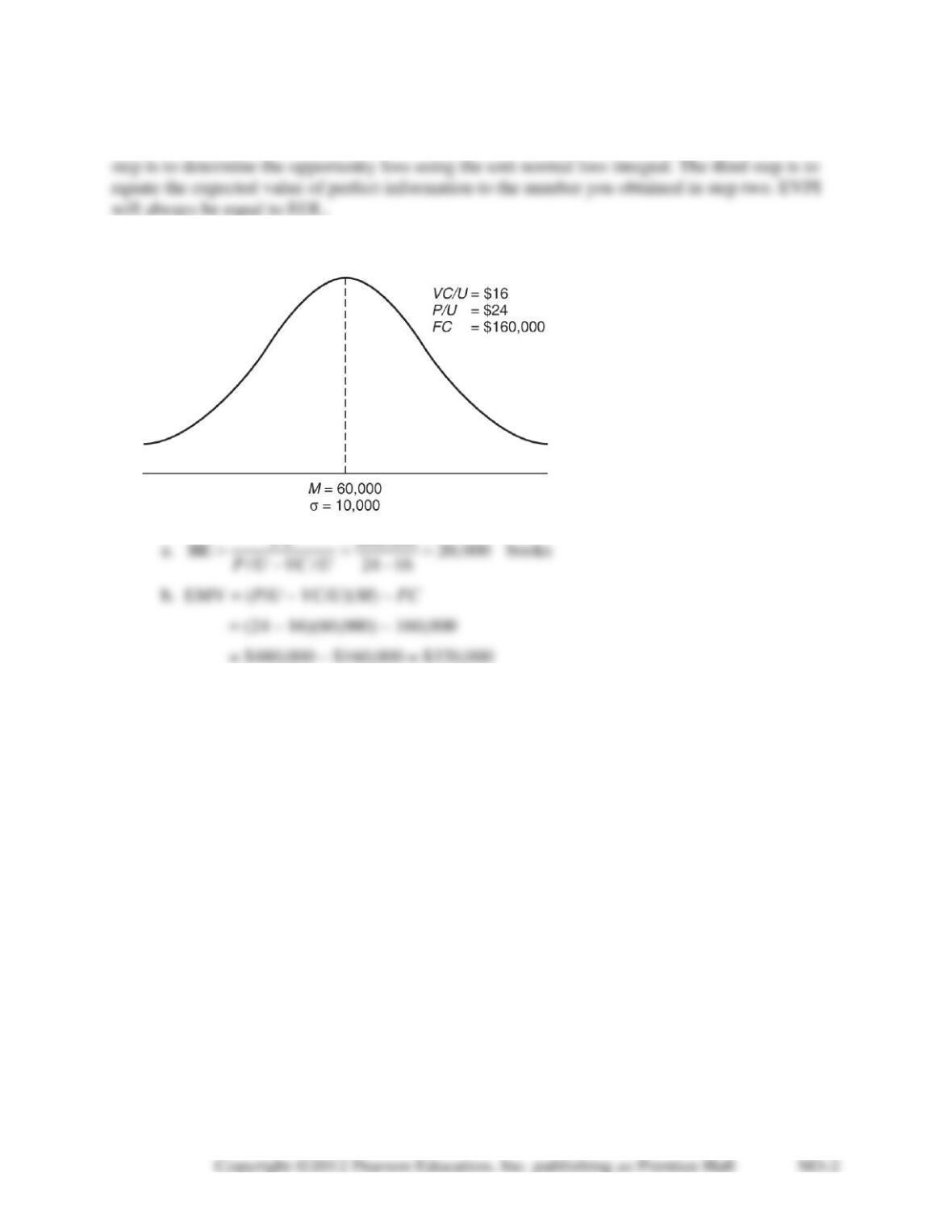
M3-8. FC = $24,000
VC/U = $8
P/U = $24
M3-9. EMV = ($28 – $20)(35,000) – $16,000
= $264,000
Standard deviation has no effect.
M3-10.
a.
OLF =
( )
$10 30 for 30 where X is
actual sales
0 otherwise
xX−
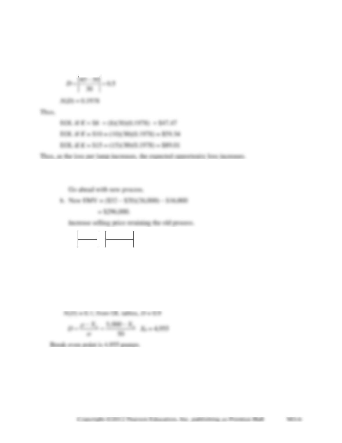
M3-11. EOL = K
N(D)
K = $8, $10, or $15
= 30
M3-12. a. New EMV = ($28 – $19)(35,000) – $32,000
= $283,000.
M3-13.
350 200 1
150
b
X
D
−−
= = =
N(D) = 0.08332
EVPI = EOL = K
N(D) = $80 150 0.08332 = $999.84
The most Joe would be willing to pay is $999.84.
M3-14. EVPI = EOL = K
N(D)
$500 = $100 50 N(D)
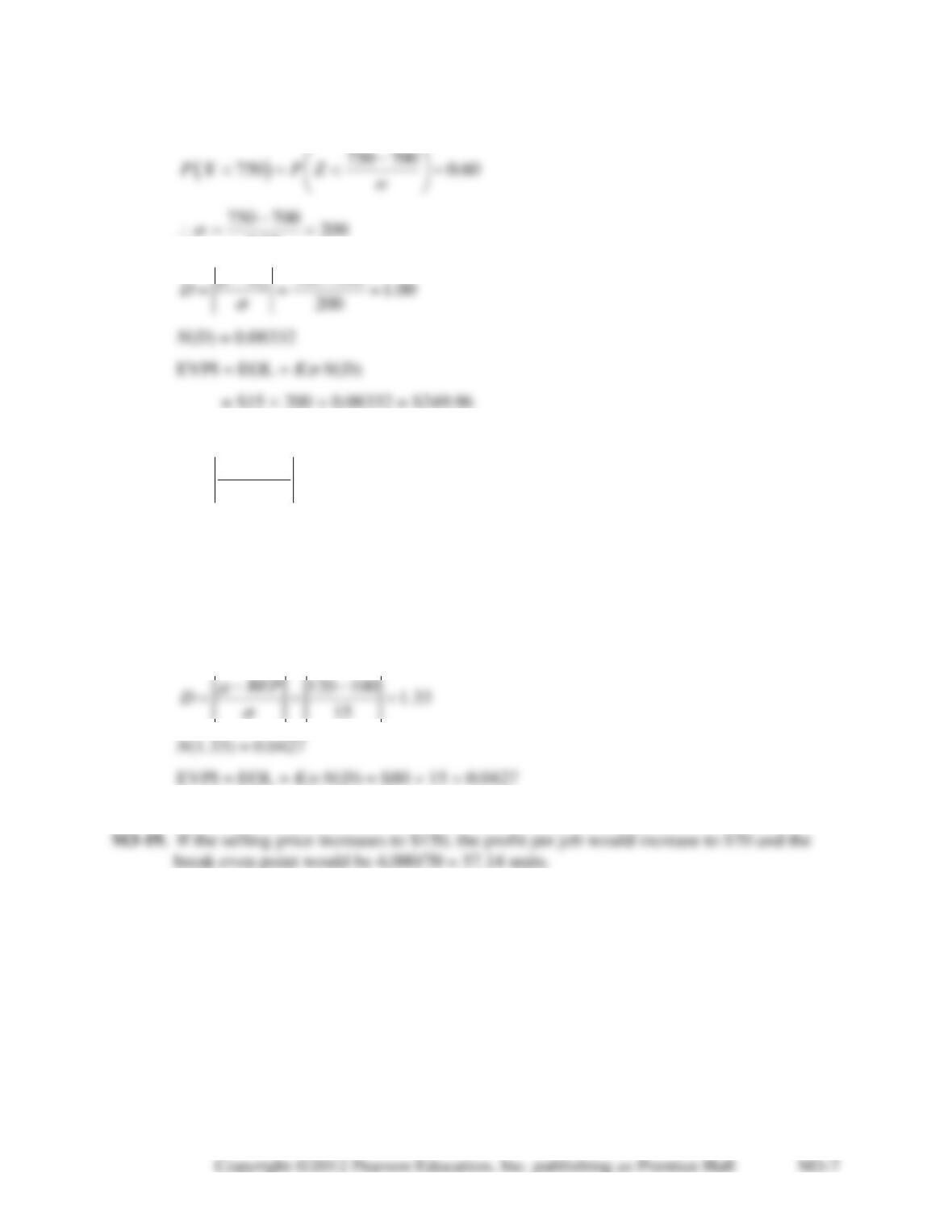
M3-15.
= 700
0.25
M3-16.
= 750;
still = 200
750 500
200
D−
=
= 1.25; N(D) decreased to 0.05059
EOL = $15 200 0.05059 = $151.77
M3-17. Fixed cost = $4,000, Profit per job = $40. Break even point = 4,000/40 = 100 jobs.
M3-18. The EVPI is equal to the minimum EOL. We use the formula
EOL = K
N(D); K = 80;
= 15; BEP = 100
= 51.24