MODULE 2
Dynamic Programming
TEACHING SUGGESTIONS
Teaching Suggestion M2.1: Overall Use of Dynamic Programming.
Dynamic programming is a general approach that can be used to solve a number of different
Teaching Suggestion M2.2: Use of the Shortest-Route Problem.
Dynamic programming can be a difficult topic for some students to understand. The shortest-
Teaching Suggestion M2.3: QA in Action Boxes in This Module.
Because dynamic programming is a difficult and advanced topic, we selected applications that
might interest the average student.
Teaching Suggestion M2.4: Use of Terminology.
Understanding dynamic programming terminology is one approach to handling larger and more
ALTERNATIVE EXAMPLE
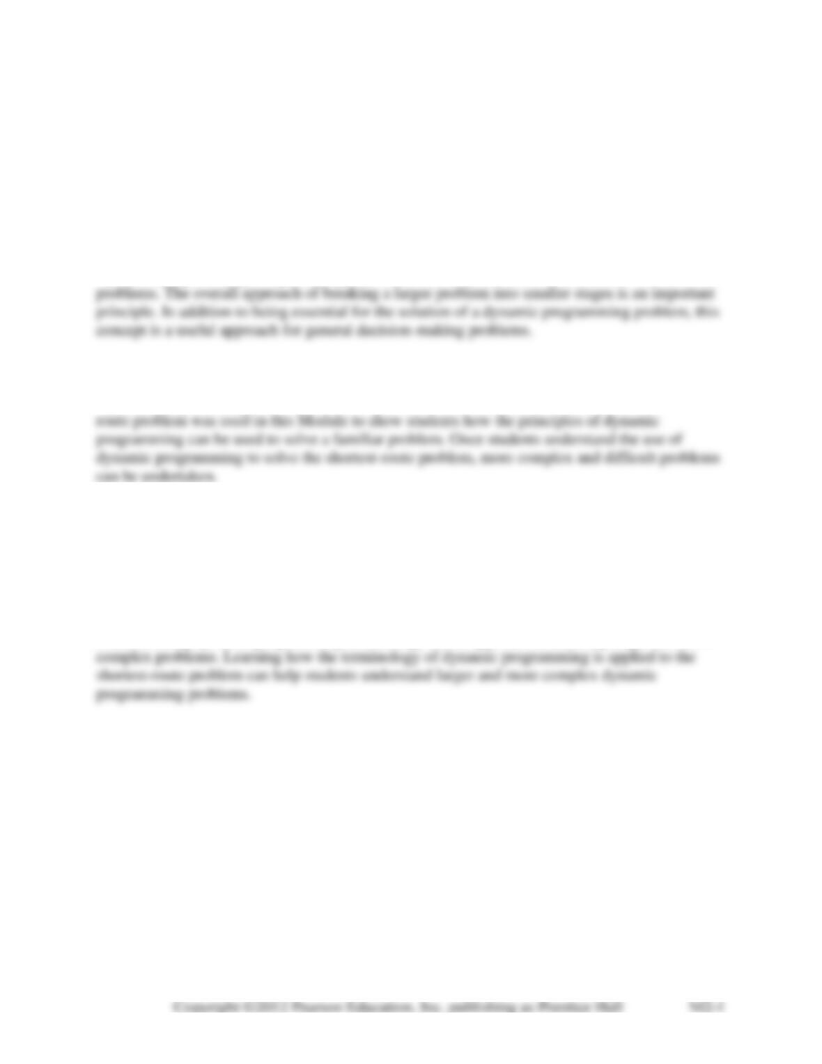
Alternative Example M2.1: Darrell Washington would like to use dynamic programming to
solve the shortest-route problem shown in the following figure.
Beginning with stage 1, we begin to solve the problem. The distance from node 5 to node 7 is 4
and the distance from node 6 is 8. These values are put in boxes by the nodes. The results are
shown in the following network.
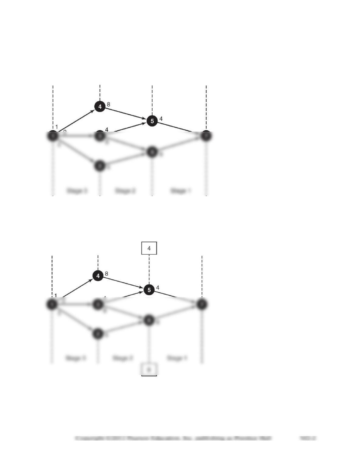
Next, we solve stage 2. The minimum distances between nodes 2, 3, and 4 and the ending node 7
are 12, 8, and 12. These distances are also put in boxes by the nodes. The results for stage 2 are
shown in the following network.
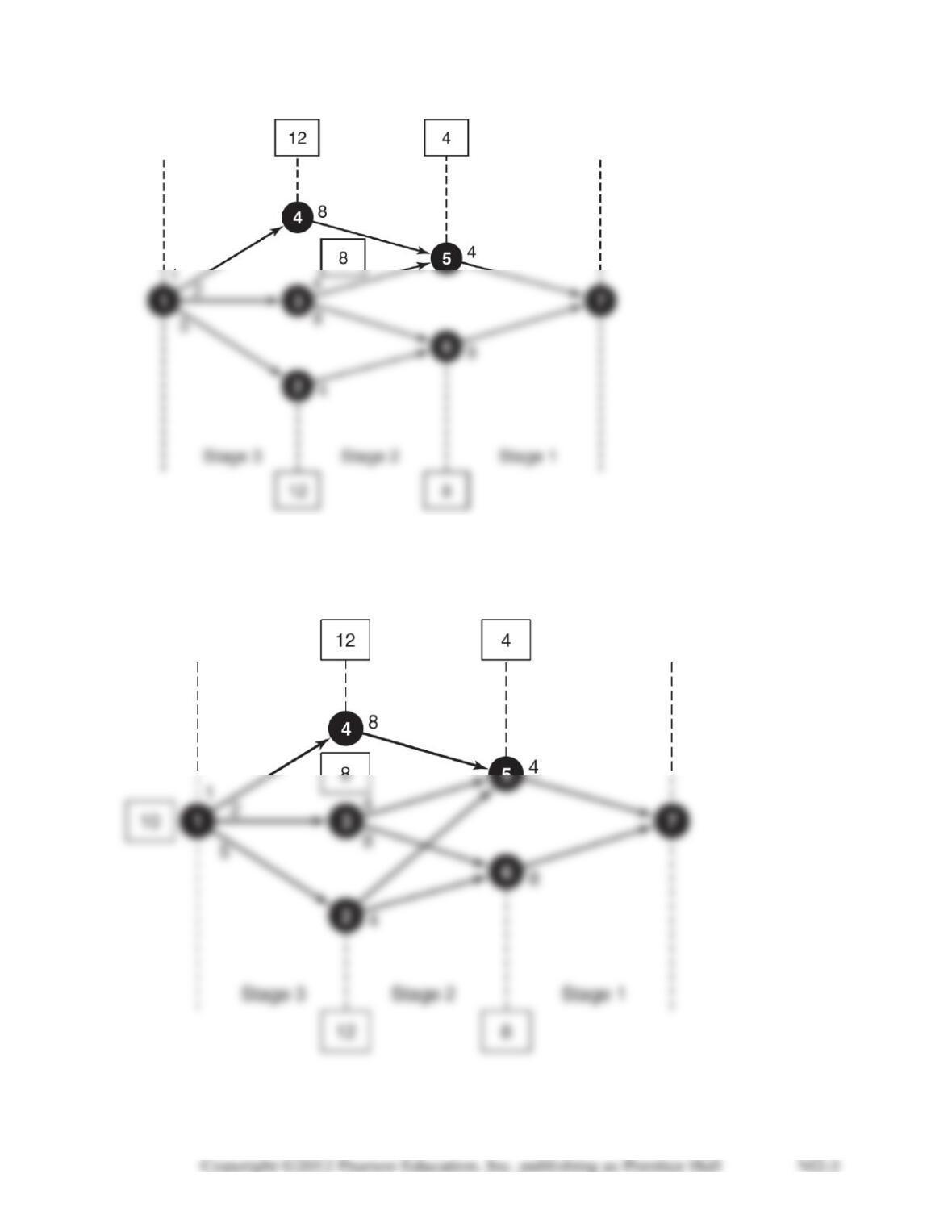
Finally, we solve stage 3. The minimum distance is through node 3. The distance from node 1 to
node 3 is 2, and the minimum distance from node 3 to the end of the network is 8 as seen in the
results for stage 2. Thus the shortest route through the network is 10.

SOLUTIONS TO QUESTIONS AND PROBLEMS
M2-1. A stage in dynamic programming is a period or a logical subproblem. Dynamic
M2-2. State variables include all of the possible beginning situations or conditions of a stage.
These have also been called the input variables. Decision variables, on the other hand, represent
M2-3. A decision criterion is a statement concerning the objective of the problem. In the
M2-4. The optimal policy is a set of decision rules, developed as a result of the decision criteria.
The optimal policy is necessary for all dynamic programming problems to give those problems
optimal decisions for any entering condition at any stage.
M2-5. A transformation is important for dynamic programming problems because it allows us to
determine the relationship between stages. This permits us to go from one stage to the next in
M2-6. The shortest route is 1–2–6–7 with a total distance of 8 miles. See the graph below.
M2-7. The shortest route is 1–2–5–7 with a total distance of 20 miles. See the graph below.
M2-8. The shortest route is 1–2–6–7 with a total distance of 14 miles. See the graph below.
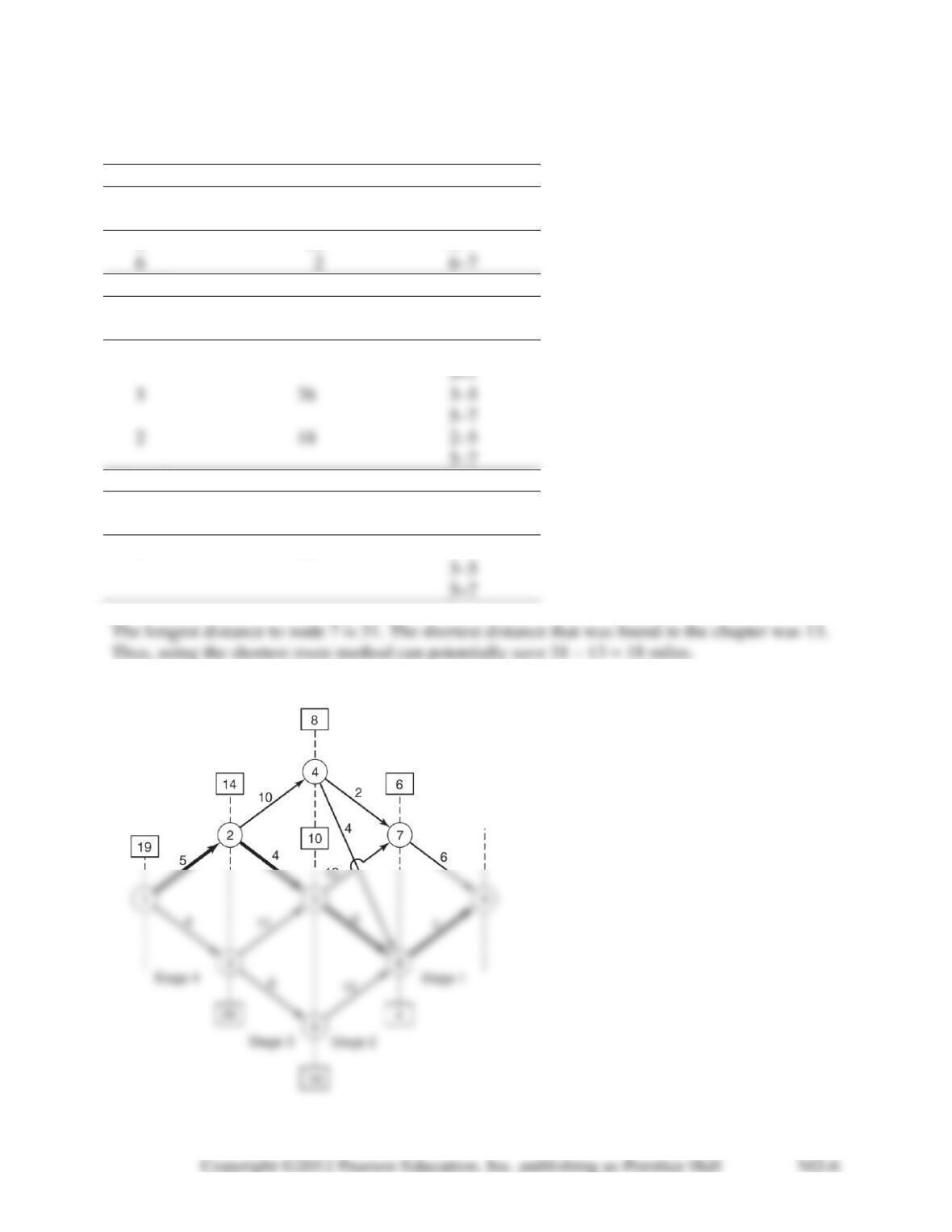
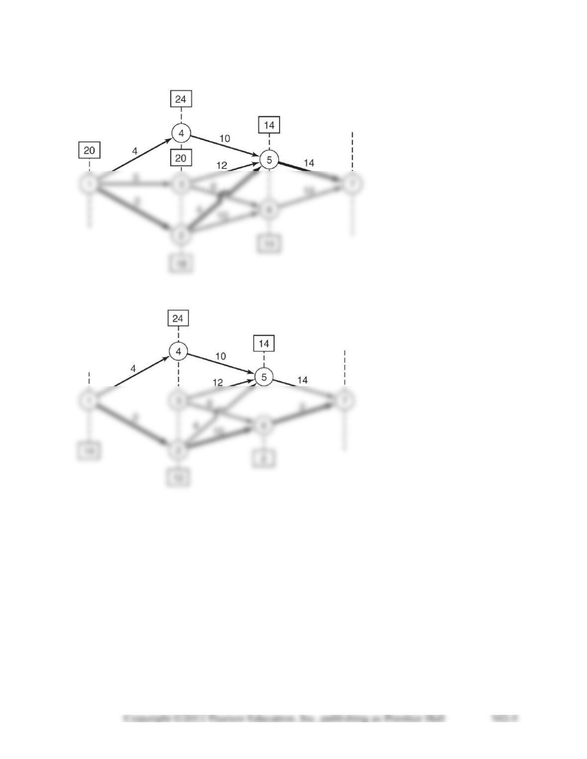
M2-9. The distances are summarized in Table M2.1. The stages are the same stages that were
used to minimize the distance.
Stage 1
Beginning
node
Longest distance
to node 7
Arcs along this
path
5
14
5–7
6
6–7
Stage 2
Beginning
node
Longest distance
to node 7
Arcs along this
path
4
24
4–5
5–7
3
26
3–5
5–7
2
18
2–5
5–7
Stage 3
Beginning
node
Longest distance
to node 7
Arcs along this
path
1
31
1–3
3–5
5–7
M2-10. The shortest route is 1–2–5–8–9 with a total distance of 19 miles. See the graph below.
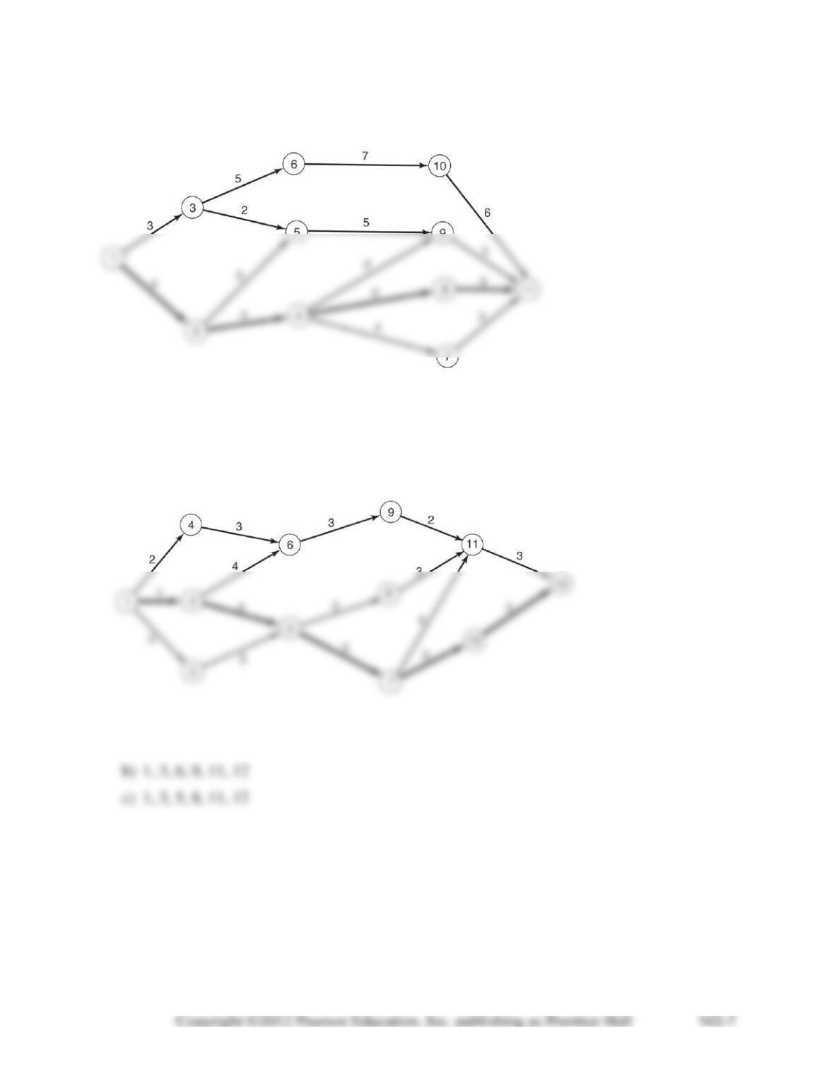
M2-11. The solution, route 1-2-4-8-11 with a total distance of 11, for this shortest-route problem
can be seen in the following network:
M2-12. The optimal decision is to ship 4 units of item 1, 1 unit of item 2, and no units of items 3
and 4.
M2-13. Given the data presented in this problem, the shortest route for Leslie is the following:
1, 3, 5, 7, 10, and 12.
Other optimal solutions for Problem M2-13 are:
a) 1, 4, 6, 9, 11, 12
M2-14. Given the data presented in this problem, the following number of units should be
shipped for each item:
Item
Items to Ship
Optimal Return
1
6
$18
2
1
9
3
1
8
4
0
0
5
0
0
6
0
8
$35
M2-15. With these changes, the new shipping pattern is:
Item
Items to Ship
Optimal Return
1
6
$18
2
1
9
3
1
8
4
0
0
5
0
0
6
2
9
$37
As you can see, the shipping pattern is slightly different.
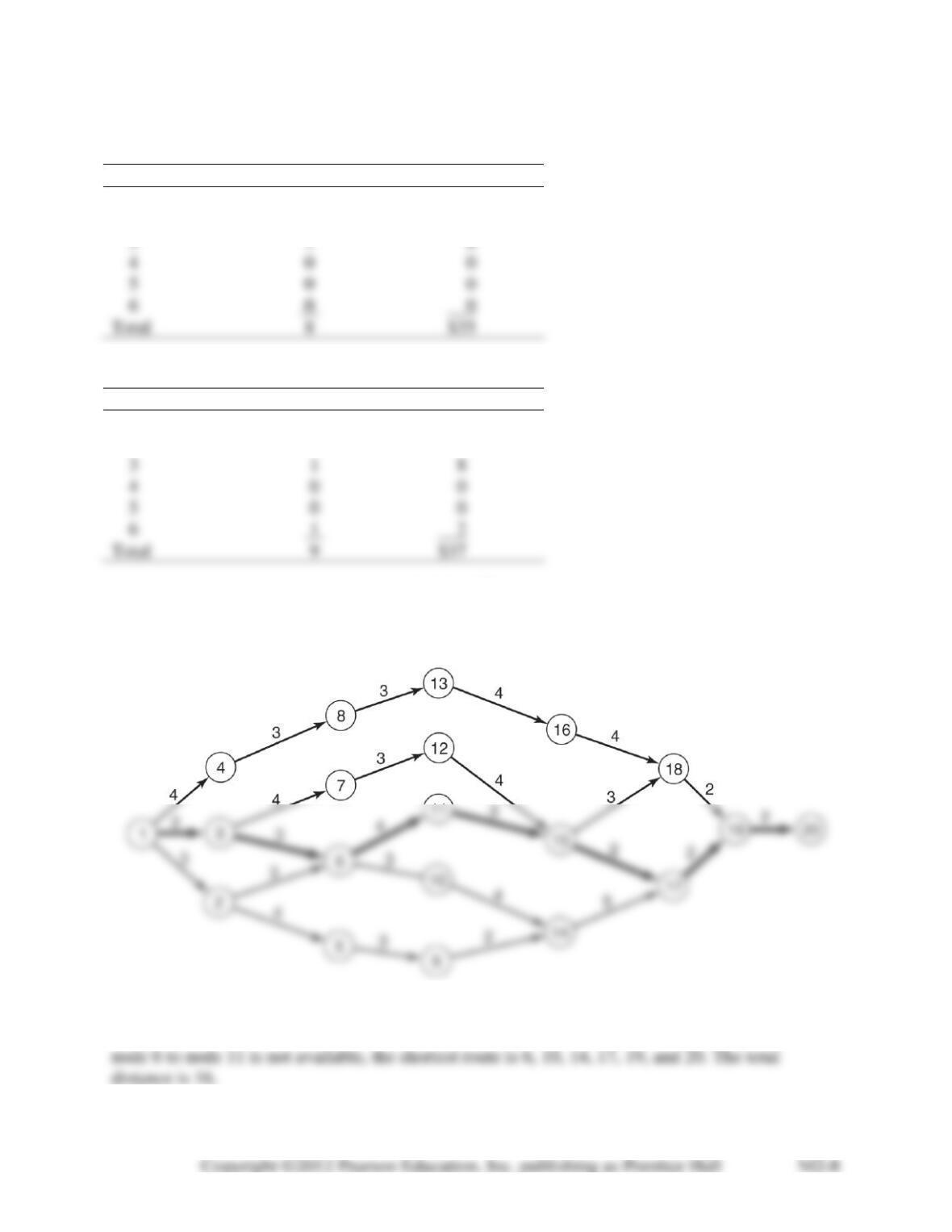
M2-16. The shortest route for this problem is 1, 3, 6, 11, 15, 17, 19, and 20 for a total distance
of 18. The optimal solution is shown in the following network.
M2-17. The optimal solution is now 1, 3, 7, 12, 15, 17, 19, and 20 for a total distance of 19.
M2-18. The shortest route is 6, 11, 15, 17, 19, and 20. The total distance is 13. If the road from
M2-19. The optimal solution is to carry 1 unit of item A and 3 units of item C. The total
nutritional value is 5,100. The total weight is 18 pounds.
SOLUTION TO UNITED TRUCKING CASE
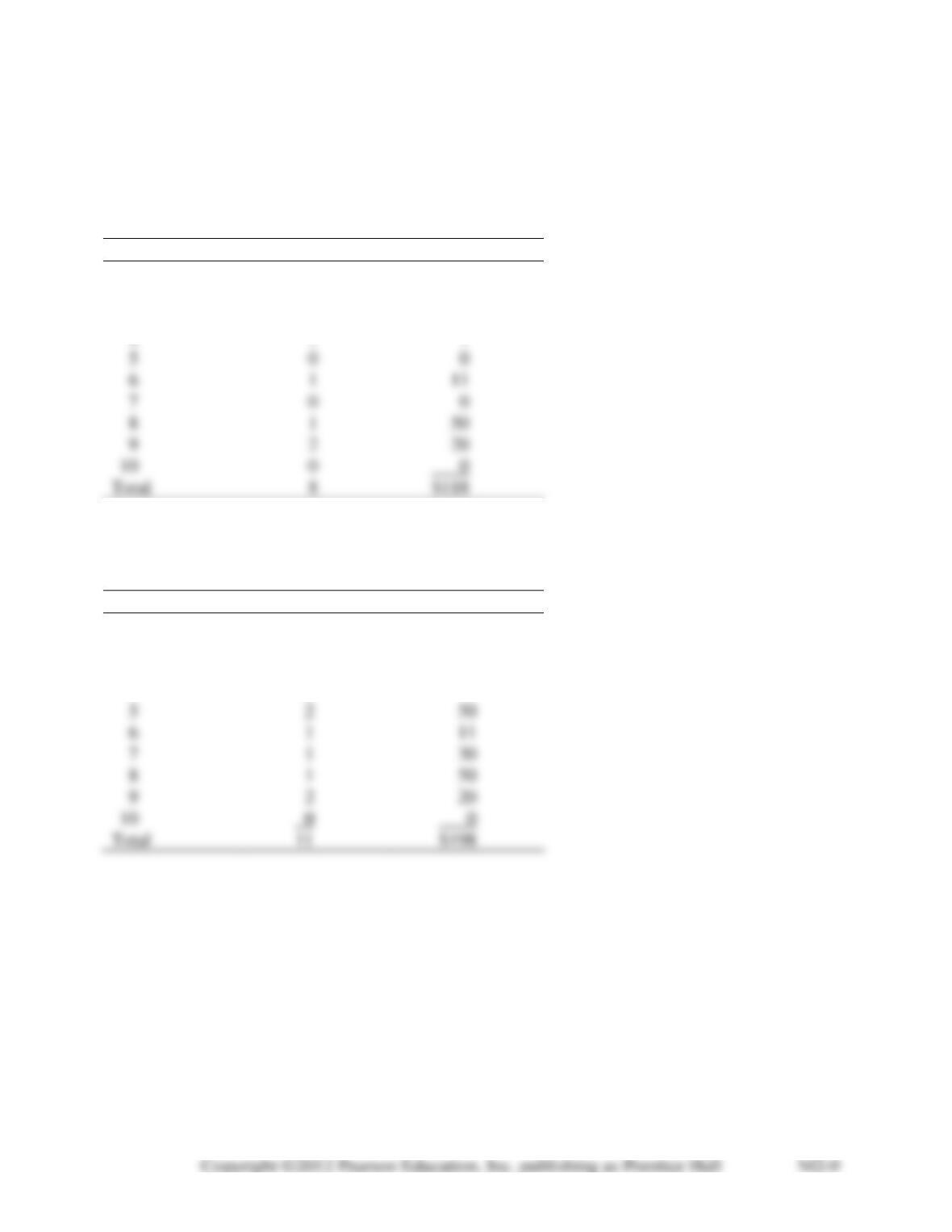
1. The optimal shipping pattern is shown in the following table.
Item
Items to Ship
Optimal Return
1
2
$20
2
1
10
3
0
0
4
1
7
5
0
0
6
1
11
7
0
0
8
1
50
9
2
20
0
8
2. Increasing the total capacity to 20 tons has a dramatic impact on the optimal decision, as can
be seen in the following table. This does include 11 items instead of 10, and assumes that the
maximum number of items increased when the weight increased.
Item
Items to Ship
Optimal Return
1
2
$20
2
1
10
3
0
0
4
1
7
5
2
50
6
1
11
7
1
30
8
1
50
9
2
20
SOLUTION TO INTERNET CASE
Briarcliff Electronics
The apportionment of the $100,000 among the various models can be accomplished by means of
dynamic programming. This can be viewed as a five stage process—at stage 1, an amount x1 is
invested in “Standard”, at stage 2, an amount x2 is invested in the “Micro” model, and so on
Define fn(x) as the maximum increased profit that can be realized over stages n through 5
given that the amount not yet invested at stage n is x. (Note that some texts number the stages
is the increased profit that would be realized over stages n through 5 if y is invested at stage n
and the remaining x – y is invested optimally over stages n + 1 through 5. Then
fn(x) = max fn(yx) = max [gn(y) + fn+1(x – y)]
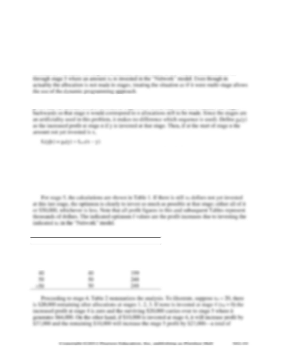
is the recursive relationship that allows one to start at stage 5 and successively determine the
optimum allocation for each stage—note that the maximization in this expression is taken over
all y x.
Table 1 Stage 5 Calculations
x5
y
f5(x5)
0
0
0
10
10
27
20
20
64
30
30
101
40
40
50
50
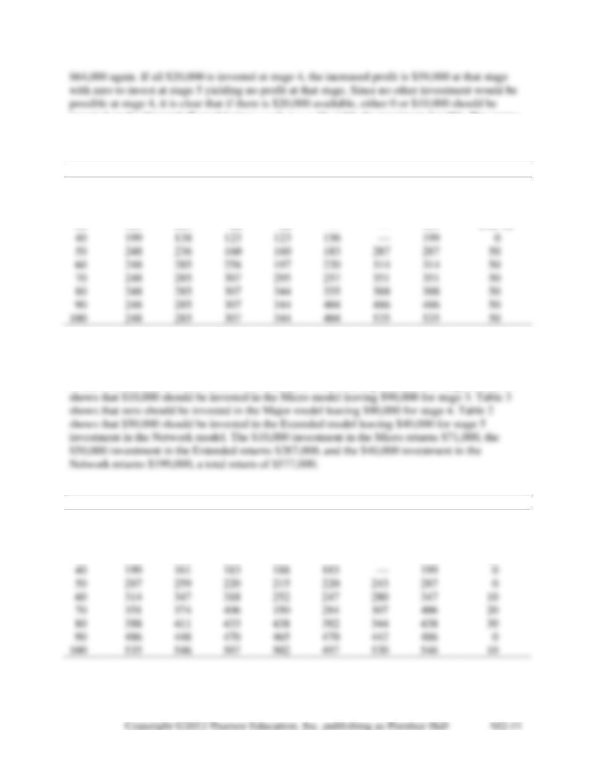
invested on the “Extended” model since y = 0 or y = 10 yields the maximum f4(y20). The entries
in the other rows are obtained in a similar manner.
Table 2 Stage 4 Calculations
x4|y
0
10
20
30
40
50
f4(yx4)
Optimal y
0
0
—
—
—
—
—
0
0
10
27
37
—
—
—
—
37
10
20
64
64
59
—
—
—
64
0 or 10
30
101
101
86
96
—
—
101
0 or 10
50
248
236
160
160
183
287
287
50
60
248
285
258
197
220
314
314
50
70
248
285
307
295
257
351
351
50
80
248
285
307
344
355
388
388
50
90
248
285
307
344
404
486
486
50
248
285
307
344
404
535
535
50
Table 3, on the previous page, shows the equivalent stage 3 calculations for the “Major”
model and Table 4 shows the stage 2 calculations for the “Micro” model. At stage 1, all
$100,000 is available. The calculations for the “Standard” model are shown in Table 5. This
reveals that zero should be invested in the Standard model leaving $100,000 for stage 2. Table 4
Table 3 Stage 3 Calculations
x3|y
0
10
20
30
40
50
f3(y|x3)
Optimal y
0
0
—
—
—
—
—
0
0
10
37
60
—
—
—
—
60
10
20
64
97
119
—
—
—
119
20
30
101
124
156
151
—
—
156
20
40
199
161
183
188
183
—
199
0
50
287
259
220
215
220
243
287
0
60
314
347
318
252
247
280
347
10
70
351
374
406
350
284
307
406
20
80
388
411
433
438
382
344
438
30
90
486
448
470
465
470
442
486
0
535
546
507
502
497
530
546
10
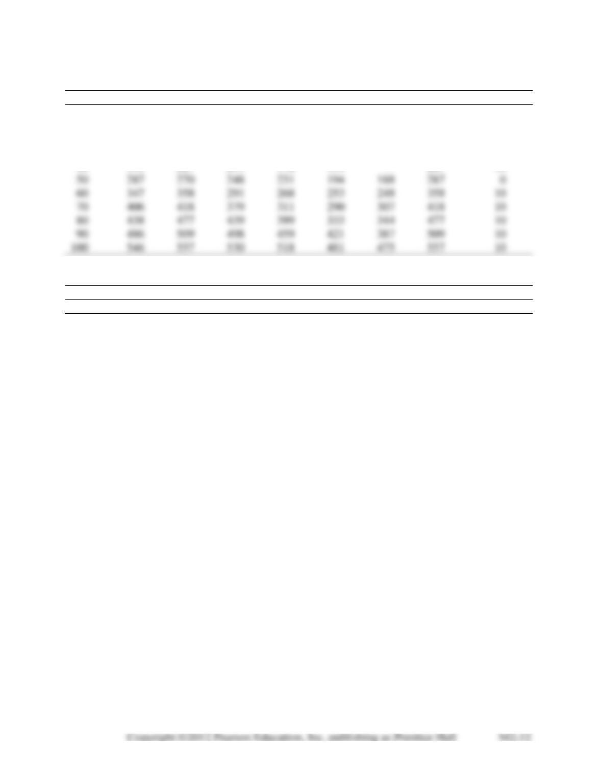
Table 4 Stage 2 Calculations
x2|y
0
10
20
30
40
50
f2(y|x2)
Optimal y
0
0
—
—
—
—
—
0
0
10
60
71
—
—
—
—
71
10
20
119
131
92
—
—
—
131
10
30
156
190
152
112
—
—
190
10
40
199
227
211
172
134
—
227
10
50
287
270
248
231
194
188
287
0
60
347
358
291
268
253
248
358
10
70
406
418
379
311
290
307
418
10
80
438
477
439
399
333
344
477
10
90
486
509
498
459
421
387
509
10
100
546
557
530
518
481
475
557
10
Table 5 Stage 1 Calculations
x1|y
0
10
20
30
40
50
f1(y|x1)
Optimal y
100
557
525
533
498
552
530
557
0