
9-1
The Time Value of Money
Author’s Overview
This is one of the most important chapters in the book as far as student comprehension is
concerned. The instructor should first determine how much prior knowledge of time value of
money the students have acquired from accounting or lower mathematics. While most students are
generally familiar with the concepts of future value and present value, they often lack the ability to
identify and categorize the nature of the problem before them.
The material in this chapter will serve as a springboard to the remaining chapters in this section on
valuation, cost of capital, and capital budgeting–related topics. A good background in time value
of money will ease the transition. The authors suggest a liberal use of homework problems and a
quiz to reinforce the importance of this material.
This chapter uses color-coordinated figures to explain the relationships between present value and
future value, present value and the present value of annuities, and future value and the future value
of annuities. These color-coded figures are helpful to those more visually oriented students who
may not understand the mathematical relationships between these time value calculations.
For faculty who want to emphasize Excel spreadsheets and calculator keystrokes, this chapter
provides an excellent opportunity to develop both skills. Using spreadsheets with time-value
exercises can be especially instructive in understanding the concept of how higher discount rates
generate lower cash flows and vice versa.
Chapter Concepts
LO1. Money has a time value associated with it, and therefore a dollar received today is worth
more than a dollar received in the future.
LO3. The present value is based on the current value of funds to be received.
9
9-2
LO5. Compounding or discounting may take place on a less than annual basis such as
semiannually or monthly.
Author’s Note:
In previous editions of Foundations of Financial Management, the authors have emphasized the
use of time value tables in the text. This has presented several problems. With the advent of
9-3
Annotated Outline and Strategy
I. Relationship to the Capital Outlay Decision: Capital budgeting involves the analysis of
whether or not funds invested today will be more than offset by the value of the funds
received from the investment in the future.
II. Future Value—Single Amount
A. In determining future value, we measure the value of an amount that is invested now
and allowed to grow at a given interest rate over a specified period of time.
B. The relationship may be expressed by the following table formula:
C. Using a financial calculator to derive the future value of a single payment, enter the
known values for the following:
N enter the number of interest periods
I/Y enter the annual interest rate
PPT Future Value of $1, FVIF = (1 + i)n (Table 9A-1)
Perspective 9-1: One or two numerical examples using this spreadsheet are helpful.
III. Present Value—Single Amount
A. The present value of a future sum is the investment required today that will equal the
future sum at a specified point in time at a given interest rate.
PPT Present Value of $1, PVIF = 1(1 + i)n (Table 9A-2)
FV = PV(1 )n
i+
FV = PV FVIF
9-4
PPT Relationship of Present Value and Future Value (Figure 9-1)
Perspective 9-2: Use Figure 9-1 to demonstrate the relationship between present and future value.
B. The relationship may be expressed in the following formula:
C. The formula may be restated as:
D. Using a financial calculator to derive the present value of a single future payment,
enter the known values for the following:
N enter the number of interest periods
I/Y enter the annual interest rate
PV leave blank
PMT enter zero
FV enter the future value amount
Then press the CPT key and then the PV key
(The resulting value will appear as a negative number.)
Perspective 9-3: We would suggest using the Excel spreadsheet example on page 261 to show the
relationship of the present value to the discount rate and time period.
IV. Interest Rate—Single Amount
A. When we know the future value, the present value, and the time period, we can
solve for the interest rate or the rate of return on an investment.
B. Using Formula 9-3 we find that:
C. We can use calculator keystrokes or the Excel spreadsheet to solve for the
1
PV = FV (1 )n
i+
PV = FV PVIF
1
FV 1
PV
n
i
=−
9-5
interest rate.
V. Number of Periods—Single Amount
A. Following up on the interest rate example, we can use Formula 9-4 to solve for the
VI. Future Value—Annuity
A. An annuity represents consecutive payments or receipts of equal amounts over equal
time intervals.
B. The annuity value is normally assumed to take place at the end of each period.
C. The future value of an annuity represents the sum of the future value of the
individual flows.
PPT Compounding Process for Annuity (Figure 9-2)
PPT Future Value of an Annuity of $1, FVIFA = [(1 + i)n – 1]/i (Table 9A-3)
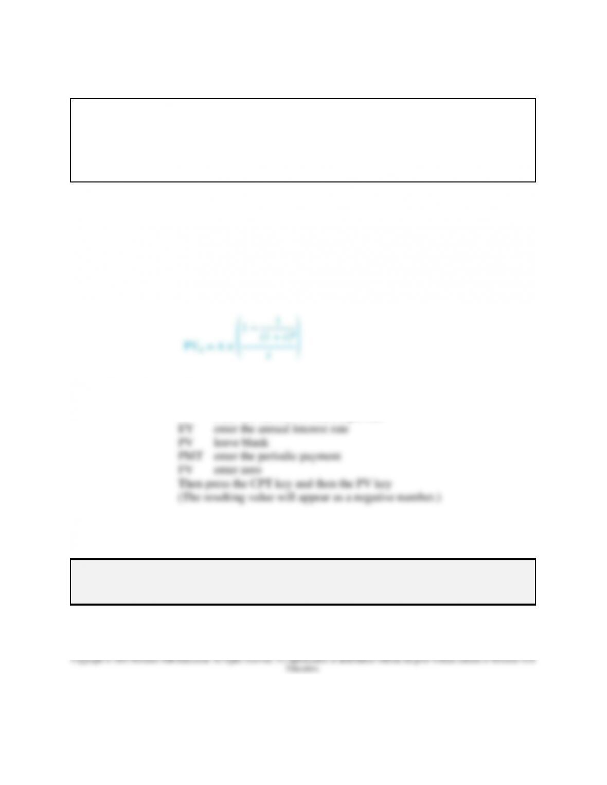
D. The formula for the future value for an annuity is given in Formula 9-5:
values for the following:
N enter the number of interest periods
9-6
(The resulting value will appear as a negative number.)
Finance in Action: Powerball Jackpot Decisions
The odds of winning are now 1 in 292 million after Powerball changed the number of choices for
the white and red numbers, and many students will be quite familiar with the $758.7 million
Powerball prize won in August 2017. However, the purpose of the box is to demonstrate the
impact that present value has on an annuity prize taken as a lump sum payout. As a sidebar, you
might want to bring in what taxes do the lump sum payout.
VII. Present Value—Annuity
A. The present value of an annuity represents the sum of the present value of the
individual cash flows.
B. The formula for the present value of an annuity is presented in Formula 9-6 (also see
Appendix D for PVIFA)
C. Using a financial calculator to derive the present value of an annuity, enter the
known values for the following:
N enter the number of interest periods
D. The annuity value associated with a present value is often associated with withdrawal
of funds from an initial deposit or the repayment of a loan.
Perspective 9-4: An example that might ring true with the students is to have them use the Excel
spreadsheet on page 267 to calculate their annual or monthly student loan repayment once they
graduate from college and have a job. It might be an eye-opening exercise.
VIII. Graphical Presentation of Time Value Relationships
A. Use Figures 9-3 and 9-4 to show that present value and future value are inversely
related.
B. Use Figures 9-5 and 9-6 to demonstrate how annuities are the sums of single period
values.
PPT Future Value of $0.68 at 10% (Figure 9-3)
PPT Present Value of $1.00 at 10% (Figure 9-4)
PPT Present Value of $1.00 at 10% (Figure 9-5)
PPT Future Value of $0.68 at 10% (Figure 9-6)
IX. Determining the Annuity Value (The amount of the periodic payment that would grow
to the requisite future value or be discounted to the requisite present value)
A. Annuity equaling a future value
1. The formula for the future value for an annuity is found in Formula 9-7:
PPT Relationship of Present Value to Annuity (Table 9-1)
Perspective 9-5: Demonstrate how annuities work in everyday situations.
PPT Payoff Table for Loan (Amortization Table) (Table 9-2)
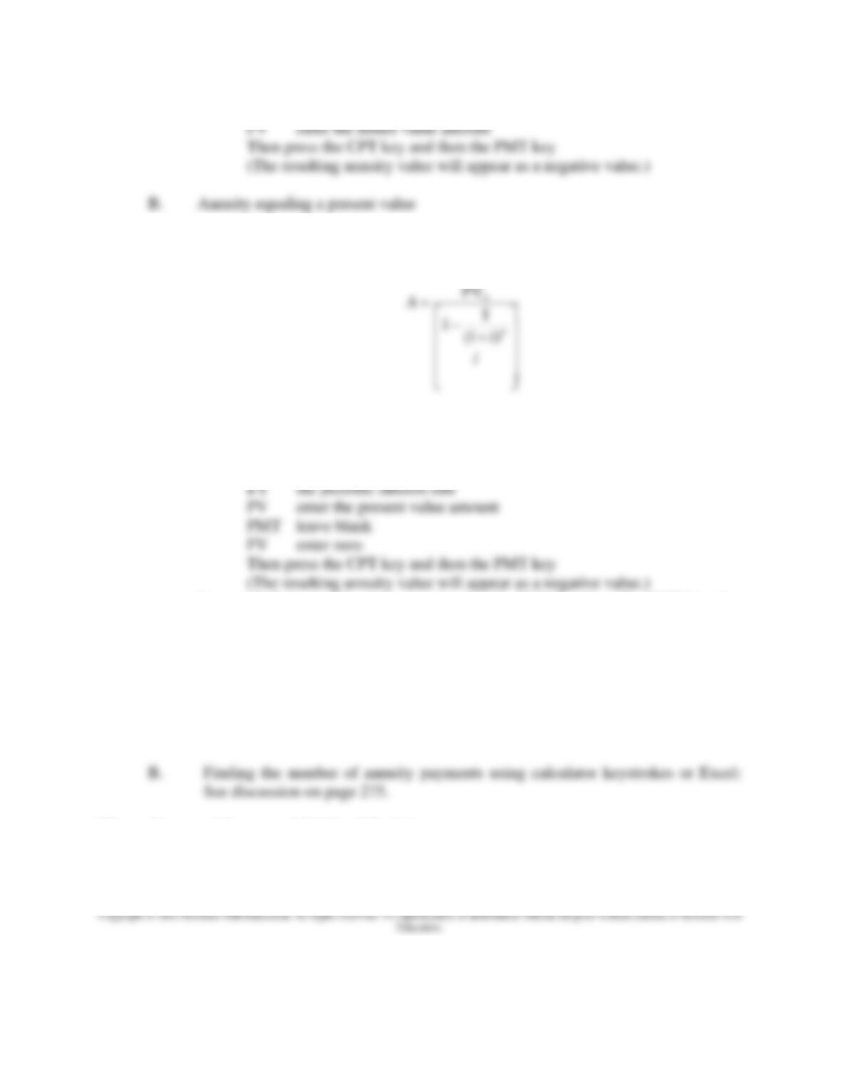
2. Using a financial calculator to derive the annuity value required to achieve a
future amount, enter the known values for the following:
FV
(1 ) 1
A
n
Ai
i
=
+−
9-8
PMT leave blank
1. The formula for the present value of an annuity is presented in Formula 9-8:
2. Using a financial calculator to derive the annuity value required to achieve a
present amount, enter the known values for the following:
N enter the number of interest periods
3. Finding annuity payments using Excel’s PMT function: The PMT function
assumes that each payment is at the end of a period. Either the PV or FV
argument must be entered. See the example on page 274.
X. Finding Interest Rates and the Number of Payments
A. Finding annuity interest rates using calculator keystrokes or Excel: See discussion
on page 274.
XI. Compounding over Additional Periods
A. Compounding semiannually requires us to cut the annual interest rate in half and to
PV
1
1(1 )
A
n
A
i
i
=
−
+
Case 2 on pages 275–276.
B. Patterns of payment with a deferred annuity: Sometimes an annuity does not start
being received until several years in the future, and under these conditions, we need
XII. Alternative Calculations: Using TVM Tables—Appendix 9A, Pages 288–291
A. Future value of a single amount
1. In determining future value, we measure the value of an amount that is
invested now and allowed to grow at a given interest rate over a specified
period of time.
2. The relationship may be expressed by the following formula:
B. Present value of a single amount
1. The present value of a future sum is the investment required today at a given
interest rate that will equal the future sum at a specified point in time.
2. The relationship may be expressed in the following formula:
PV = FV 1
(1+in
)
C. Future value of an annuity
1. An annuity represents consecutive payments or receipts of equal amounts
over equal time intervals.
FV = PV(1 )n
i+
FV = PV FVIF

9-10
period.
4. The formula for the future value for an annuity is:
FVA = A FVIFA
D. Present value of an annuity
1. The present value of an annuity represents the sum of the present value of the
individual cash flows.
2. The formula for the present value of an annuity is:
PVA = A PVIFA
Other Chapter Supplements
Cases for Use with Foundations of Financial Management
Case 11, Billy Wilson, All American (time value of money)